<?xml version="1.0" encoding="ISO-8859-1"?><article xmlns:mml="http://www.w3.org/1998/Math/MathML" xmlns:xlink="http://www.w3.org/1999/xlink" xmlns:xsi="http://www.w3.org/2001/XMLSchema-instance">
<front>
<journal-meta>
<journal-id>1012-7089</journal-id>
<journal-title><![CDATA[Terra]]></journal-title>
<abbrev-journal-title><![CDATA[Terra]]></abbrev-journal-title>
<issn>1012-7089</issn>
<publisher>
<publisher-name><![CDATA[Instituto de Geografía y Desarrollo Regional y de los Postgrado en Geografía, FHE, UCV]]></publisher-name>
</publisher>
</journal-meta>
<article-meta>
<article-id>S1012-70892010000100003</article-id>
<title-group>
<article-title xml:lang="es"><![CDATA[Determinación del tipo de régimen de lluvia anual en estaciones pluviométricas venezolanas, según análisis de Fourier y el análisis de grupo]]></article-title>
<article-title xml:lang="en"><![CDATA[Rain Annual Rate Regime of a set of Venezuelan Rainfall Stations, Based on Fourier Analysis, and the Analysis of Group]]></article-title>
</title-group>
<contrib-group>
<contrib contrib-type="author">
<name>
<surname><![CDATA[Blanco]]></surname>
<given-names><![CDATA[Andrés]]></given-names>
</name>
<xref ref-type="aff" rid="A01"/>
</contrib>
<contrib contrib-type="author">
<name>
<surname><![CDATA[Barboza]]></surname>
<given-names><![CDATA[Jesús]]></given-names>
</name>
<xref ref-type="aff" rid="A01"/>
</contrib>
<contrib contrib-type="author">
<name>
<surname><![CDATA[Rodríguez]]></surname>
<given-names><![CDATA[Jorge]]></given-names>
</name>
<xref ref-type="aff" rid="A01"/>
</contrib>
</contrib-group>
<aff id="A01">
<institution><![CDATA[,UCV Escuela de Geografía ]]></institution>
<addr-line><![CDATA[ ]]></addr-line>
</aff>
<pub-date pub-type="pub">
<day>00</day>
<month>06</month>
<year>2010</year>
</pub-date>
<pub-date pub-type="epub">
<day>00</day>
<month>06</month>
<year>2010</year>
</pub-date>
<volume>26</volume>
<numero>39</numero>
<fpage>31</fpage>
<lpage>57</lpage>
<copyright-statement/>
<copyright-year/>
<self-uri xlink:href="http://ve.scielo.org/scielo.php?script=sci_arttext&amp;pid=S1012-70892010000100003&amp;lng=en&amp;nrm=iso"></self-uri><self-uri xlink:href="http://ve.scielo.org/scielo.php?script=sci_abstract&amp;pid=S1012-70892010000100003&amp;lng=en&amp;nrm=iso"></self-uri><self-uri xlink:href="http://ve.scielo.org/scielo.php?script=sci_pdf&amp;pid=S1012-70892010000100003&amp;lng=en&amp;nrm=iso"></self-uri><abstract abstract-type="short" xml:lang="es"><p><![CDATA[Para describir el régimen climático de precipitación intra-anual, generalmente se identifican los lapsos de valores mayores y menores a la media aritmética de los 12 valores mensuales, así como los montos pluviales extremos. Este trabajo tiene como finalidad configurar la variación de la lluvia en el año aplicando el Análisis de Fourier a los registros climáticos correspondientes al lapso 1961-1990, a 15 estaciones pluviométricas distribuidas en el territorio nacional, para, posteriormente, agruparlas en conjuntos internamente homogéneos pero externamente heterogéneos utilizando la técnica de agrupación automática (Cluster Análisis). La obtención de los coeficientes de Fourier, generó una matriz de 15 casos por 6 valores asociados a las curvas armónicas de tres ciclos, valores correspondientes a las amplitudes y ángulos de fases de dichas funciones periódicas, y explican más del 90% de la variabilidad mensual de la lluvia, así se obtuvieron siete grupos: (1) Barcelona, Ciudad Bolívar, Maturín, San Fernando de Apure, con un régimen pluvial unimodal y máximo en julio-agosto; (2) Barquisimento, Santa Elena de Uairén, con máximo en junio y otro secundario en octubre; (3) Colonia Tovar, Maracaibo, Maracay, Mene Grande con máximos en septiembre-octubre y otro máximo secundario en mayo-junio; (4) Coro, Maiquetía con un régimen de lluvia que se incrementa desde febrero y marzo hasta fines de año; (5) Mérida con régimen bimodal con máximos en Mayo y Octubre con mínimo secundario en julio; (6) Puerto Ayacucho con régimen pluvial unimodal con máximo en junio y extremo mínimo por encima de los 30 mm y (7) San Antonio del Táchira tiene un régimen bimodal con máximos en abril y octubre y mínimo secundario que comprende los meses de Julio y Agosto. Al comparar los resultados de agrupación con los pluviogramas se constató que su representación mediante los coeficientes de Fourier fue adecuada, concluyéndose que puede sugerirse como una opción para incluir la condición de variabilidad pluvial anual.]]></p></abstract>
<abstract abstract-type="short" xml:lang="en"><p><![CDATA[To describe the climate regime of intra-annual precipitation, generally identified lapses greater and less than the arithmetic mean of the 12 monthly values and extreme rainfall amounts. This paper aims to set the variation of rainfall in the year by applying Fourier analysis to the climate record, covering the period 1961-1990, 15 rainfall stations distributed over the national territory, and then combined into groups internally homogeneous but externally heterogeneous using automatic clustering technique (Cluster Analysis). Obtaining the Fourier coefficients by multiple regression, generated a matrix of 15 cases for 6 values associated with three cycles of harmonic curves, which at least explained in more 90% of the variability of monthly rainfall. In this way were seven groups, namely: (1) Barcelona, Ciudad Bolívar, Maturín, San Fernando de Apure, which are characterized by a unimodal rainfall regime with a peak in july-August (2) Barquisimento, Santa Elena de Uairén, with maximum in june and october secondary, (3) Colonia Tovar, Maracaibo, Maracay, Mene Grande peaks in september-october and another secondary maximum in may-june (4) Coro, Maiquetía with a rain which increased from february and march until the end of the year (5) Merida presents a bimodal peaks in may and in october with minimal side july (6) Puerto Ayacucho with unimodal rainfall regime with maximum in june and far above the minimum of 30 mm and (7) San Antonio del Tachira has a bimodal peaks in april and october and lower secondary which covers the months of july and august. Comparing these results with the automatic grouping respective pluviogramas was found that the representation by means of Fourier coefficients was properly concluded that it may be suggested as a choice to include the status of annual rainfall variability.]]></p></abstract>
<kwd-group>
<kwd lng="es"><![CDATA[Lluvia]]></kwd>
<kwd lng="es"><![CDATA[clima]]></kwd>
<kwd lng="es"><![CDATA[régimen]]></kwd>
<kwd lng="es"><![CDATA[análisis de Fourier]]></kwd>
<kwd lng="es"><![CDATA[análisis de agrupamiento]]></kwd>
<kwd lng="es"><![CDATA[Venezuela]]></kwd>
<kwd lng="en"><![CDATA[Rain]]></kwd>
<kwd lng="en"><![CDATA[Climate]]></kwd>
<kwd lng="en"><![CDATA[Regime]]></kwd>
<kwd lng="en"><![CDATA[Fourier Analysis]]></kwd>
<kwd lng="en"><![CDATA[Cluster Analysis]]></kwd>
<kwd lng="en"><![CDATA[Venezuela]]></kwd>
</kwd-group>
</article-meta>
</front><body><![CDATA[ <p style="text-autospace: none" align="center"><font face="Verdana"><b> <span style="font-family: TimesNewRoman\,Bold">Determinación del tipo de régimen  de lluvia anual en estaciones pluviométricas venezolanas, según análisis de  Fourier y el análisis de grupo*</span></b></font></p>     <p style="text-autospace: none" align="center"><font face="Verdana"><b> <span lang="EN-US" style="font-family: TimesNewRoman">Rain Annual Rate Regime of  a set of Venezuelan Rainfall Stations, Based on Fourier Analysis, and the  Analysis of Group</span></b></font></p>     <p style="text-autospace: none" align="center"><font face="Verdana" size="2"><b> <span lang="PT-BR" style="font-family: TimesNewRoman\,BoldItalic">Andrés Blanco,  Jesús Barboza, Jorge Rodríguez</span></b></font></p>     <p style="text-autospace: none" align="justify"><font face="Verdana" size="2"> <b>Andrés E. Blanco T.</b> Licenciado en Geografía (2000) Especialista en  Análisis de Datos en Ciencia Sociales (escolaridad completa) Profesor Instructor  por Concurso (2007) Escuela de Geografía UCV. Área de Investigación:  Climatología Básica y Aplicada. Modelos Lineales, Univariados y Multivartiados;  Series de Tiempo. Correo electrónico: <a href="mailto:andeloblant@yahoo.com"> andeloblant@yahoo.com</a>.</font></p>     <p style="text-autospace: none" align="justify"><font face="Verdana" size="2"> <b>Jesús L. Barboza.</b> Licenciado en Geografía (2000). Profesor Instructor  Escuela de Geografía UCV. Área de Investigación: Climatología Básica y Aplicada.  Modelos Lineales, Univariados y Multivartiados; Series de Tiempo. Correo  electrónico: <a href="mailto:jlubarbo@yahoo.com">jlubarbo@yahoo.com</a>.</font></p>     <p style="text-autospace: none" align="justify"><font face="Verdana" size="2"> <b>Jorge Armando Rodríguez Gómez.</b> Licenciado en Geografía, Mención  Cartografía (1968, UCV). Ingeniero Civil, Mención Estructuras (1983, USM).  Magíster Scientiarum en Geografía (1986, UCV) Especialista en Planificación e  Ingeniería de los Recursos Hidráulicos (1991, USB). Profesor Titular (2000)  Escuela de Geografía UCV. Docencia en Matemáticas (USB). Maestría en Estadística  (escolaridad completa) Especialista en Análisis de Datos en Ciencia Sociales  (2004, UCV). Área de Investigación: Climatología Básica y Aplicada. Modelos  Lineales, Univariados y Multivartiados; Series de Tiempo. Correo electrónico: <a href="mailto:jarpine@yahoo.es">jarpine@yahoo.es</a>.</font></p>     <p style="text-align: justify; text-autospace: none"><font face="Verdana"><b> <span style="font-family: TimesNewRoman\,Bold"><font size="2">RESUMEN</font></span></b></font></p>     <p style="text-align: justify; text-autospace: none"><font face="Verdana"> <span style="font-family: TimesNewRoman"><font size="2">Para describir el  régimen climático de precipitación intra-anual, generalmente se identifican los  lapsos de valores mayores y menores a la media aritmética de los 12 valores  mensuales, así como los montos pluviales extremos. Este trabajo tiene como  finalidad configurar la variación de la lluvia en el año aplicando el Análisis  de Fourier a los registros climáticos correspondientes al lapso 1961-1990, a 15  estaciones pluviométricas distribuidas en el territorio nacional, para,  posteriormente, agruparlas en conjuntos internamente homogéneos pero  externamente heterogéneos utilizando la técnica de agrupación automática (</font></span><i><span style="font-family: TimesNewRoman\,Italic"><font size="2">Cluster  Análisis)</font></span></i><span style="font-family: TimesNewRoman"><font size="2">.  La obtención de los coeficientes de Fourier, generó una matriz de 15 casos por 6  valores asociados a las curvas armónicas de tres ciclos, valores  correspondientes a las amplitudes y ángulos de fases de dichas funciones  periódicas, y explican más del 90% de la variabilidad mensual de la lluvia, así  se obtuvieron siete grupos: (1) </font></span><i> <span style="font-family: TimesNewRoman\,Italic"><font size="2">Barcelona,  Ciudad Bolívar, Maturín, San Fernando de Apure</font></span></i><span style="font-family: TimesNewRoman"><font size="2">,  con un régimen pluvial unimodal y máximo en julio–agosto; (2) </font></span><i> <span style="font-family: TimesNewRoman\,Italic"><font size="2">Barquisimento,  Santa Elena de Uairén</font></span></i><span style="font-family: TimesNewRoman"><font size="2">,  con máximo en junio y otro secundario en octubre; (3) </font></span><i> <span style="font-family: TimesNewRoman\,Italic"><font size="2">Colonia Tovar,  Maracaibo, Maracay, Mene Grande </font></span></i> <span style="font-family: TimesNewRoman"><font size="2">con máximos en  septiembre-octubre y otro máximo secundario en mayo-junio; (4) Coro, Maiquetía  con un régimen de lluvia que se incrementa desde febrero y marzo hasta fines de  año; (5) </font></span><i><span style="font-family: TimesNewRoman\,Italic"> <font size="2">Mérida </font></span></i> <span style="font-family: TimesNewRoman"><font size="2">con régimen bimodal con  máximos en Mayo y Octubre con mínimo secundario en julio; (6) </font></span><i> <span style="font-family: TimesNewRoman\,Italic"><font size="2">Puerto Ayacucho </font></span></i><span style="font-family: TimesNewRoman"><font size="2">con  régimen pluvial unimodal con máximo en junio y extremo mínimo por encima de los  30 mm y (7) </font></span><i><span style="font-family: TimesNewRoman\,Italic"> <font size="2">San Antonio del Táchira </font></span></i> <span style="font-family: TimesNewRoman"><font size="2">tiene un régimen bimodal  con máximos en abril y octubre y mínimo secundario que comprende los meses de  Julio y Agosto. Al comparar los resultados de agrupación con los pluviogramas se  constató que su representación mediante los coeficientes de Fourier fue  adecuada, concluyéndose que puede sugerirse como una opción para incluir la  condición de variabilidad pluvial anual.</font></span></font></p>     <p style="text-align: justify; text-autospace: none"><font face="Verdana"><b> <span style="font-family: TimesNewRoman\,Bold"><font size="2">PALABRAS CLAVE</font></span></b><span style="font-family: TimesNewRoman"><font size="2">:  Lluvia, clima, régimen, análisis de Fourier, análisis de agrupamiento,  Venezuela.</font></span></font></p>     <p style="text-align: justify; text-autospace: none"><font face="Verdana"><b> <span lang="EN-US" style="font-family: TimesNewRoman\,Bold"><font size="2">A</font><font size="2">BSTRACT</font></span></b></font></p>     ]]></body>
<body><![CDATA[<p style="text-align: justify; text-autospace: none"> <font face="Verdana" size="2"> <span lang="EN-US" style="font-family: TimesNewRoman">To describe the climate  regime of intra-annual precipitation, generally identified lapses greater and  less than the arithmetic mean of the 12 monthly values and extreme rainfall  amounts. This paper aims to set the variation of rainfall in the year by  applying Fourier analysis to the climate record, covering the period 1961-1990,  15 rainfall stations distributed over the national territory, and then combined  into groups internally homogeneous but externally heterogeneous using automatic  clustering technique (Cluster Analysis). Obtaining the Fourier coefficients by  multiple regression, generated a matrix of 15 cases for 6 values associated with  three cycles of harmonic curves, which at least explained in more 90% of the  variability of monthly rainfall. In this way were seven groups, namely: (1)  Barcelona, Ciudad Bolívar, Maturín, San Fernando de Apure, which are  characterized by a unimodal rainfall regime with a peak in july-August (2)  Barquisimento, Santa Elena de Uairén, with maximum in june and october  secondary, (3) Colonia Tovar, Maracaibo, Maracay, Mene Grande peaks in  september-october and another secondary maximum in may-june (4) Coro, Maiquetía  with a rain which increased from february and march until the end of the year  (5) Merida presents a bimodal peaks in may and in october with minimal side july  (6) Puerto Ayacucho with unimodal rainfall regime with maximum in june and far  above the minimum of 30 mm and (7) San Antonio del Tachira has a bimodal peaks  in april and october and lower secondary which covers the months of july and  august. Comparing these results with the automatic grouping respective  pluviogramas was found that the representation by means of Fourier coefficients  was properly concluded that it may be suggested as a choice to include the  status of annual rainfall variability.</span></font></p>     <p style="text-align: justify; text-autospace: none"><font face="Verdana"><b> <span style="font-family: TimesNewRoman\,Bold"><font size="2">KEYWORDS</font></span></b><span style="font-family: TimesNewRoman"><font size="2">:  Rain, Climate, Regime, Fourier Analysis, Cluster Analysis, Venezuela.</font></span></font></p>     <p style="text-align: justify; text-autospace: none"> <font face="Verdana" size="2">* Recibido: 21-03-2009.</font></p>     <p style="text-align: justify; text-autospace: none"> <font face="Verdana" size="2">Aceptado: 15-10-2009.</font></p>      <p align="justify"><font face="Verdana" size="2"><b>PRESENTACIÓN</b></font></p>     <p align="justify"><font face="Verdana" size="2">La determinación del régimen  pluvial anual consiste en identificar la estacionalidad de la lluvia, al señalar  los máximos y mínimos relativos así como la ubicación y duración de los lapsos  lluviosos y no lluviosos. Por ejemplo, una estrategia a seguir es aplicar los  criterios del sistema de clasificación climática de Köeppen, el cual considera  hasta, distintivamente, tres regímenes: (1) con máximo o máximos en posición  astronómica alta de sol (régimen w); (2) con máximo o máximos en posición  astronómica baja de sol (régimen s) y (3) sin diferencia significativa de  períodos pluviales (régimen f);. de este modo, el régimen pluvial de la estación  La Carlota (Distrito Capital) es de carácter unimodal con máximo en el mes de  junio, mientras que la estación Observatorio Cagigal es unimodal con máximo en  el mes de octubre.</font></p>     <p align="justify"><font face="Verdana" size="2">Tal información no es adecuada  para incorporarla a una base geográfica de datos por ser incompleta, ya que no  aclara acerca de lo acontecido en la pluviosidad en el resto del año. Ello  plantea la disyuntiva de incluir, al menos, los doce datos climáticos de la  lluvia o bien realizar parámetros, mediante algún procedimiento, tal  comportamiento pluvial anual con una menor cantidad de índices, de modo que tal  síntesis no implique una pérdida significativa de la información original.</font></p>     <p align="justify"><font face="Verdana" size="2">En otro orden de ideas, la  literatura matemático-estadística plantea que el Análisis Fourier, tanto de  procesos periódicos o no, es pertinente para desagregar los componentes que  determinan una curva compleja en el dominio del tiempo. La descomposición de la  curva original en sus componentes, llamados armónicos, permite, simultáneamente,  estimar la contribución de los distintos regímenes que intervienen en la curva  original y, así mismo, indexar numéricamente cada armónico mediante los  coeficientes binómicos Fourier o bien con los coeficientes polares Fourier.</font></p>     <p align="justify"><font face="Verdana" size="2">El Análisis Fourier permite  desagregar los componentes (armónicos) que determinan una curva compleja, con  los cuales se estima la contribución de los distintos subregímenes que  intervienen en la curva original e indexar cada armónico mediante sus  coeficientes Fourier. En ese orden de ideas, Kyrkyla y Hameed. (1989), en  Estados Unidos de América, y Rodríguez (2003), en la región norte de Venezuela,  separan matemáticamente los componentes estacionales que contribuyen con la  configuración de la curva intra-anual pluviométrica de un conjunto de sitios de  medición con distribución espacial irregular. Ahora bien, dado que la curva  pluvial climática tiene 12 valores (uno por cada mes), se pueden generar,  máximo, 11 coeficientes Fourier (ó 5 armónicos). Pero, según criterio del  investigador, es factible reducir el número de armónicos a 3 ó menos, lográndose  una solución más parsimoniosa que la información pluvial original.</font></p>     <p align="justify"><font face="Verdana" size="2">En consecuencia, si la curva  pluvial original tiene 12 valores, es posible generar, hasta un máximo, de 11  coeficientes Fourier, apreciándose que la reducción de valores solamente es de  una unidad.</font></p>     ]]></body>
<body><![CDATA[<p align="justify"><font face="Verdana" size="2">Sin embargo, es posible  cuantificar la contribución a la varianza muestral total de cada armónico, y  determinar de modo aproximado, si esa contribución es estadísticamente  significativa. Por lo tanto, es factible que el número de armónicos  significativos sean tres o menos, reduciéndose así el número de coeficientes a  seis, un 50% de la información pluvial original.</font></p>     <p align="justify"><font face="Verdana" size="2">A tal efecto, este estudio se  planteó, a partir de una base de datos climáticos mensuales pluviales,  provenientes de un conjunto de estaciones venezolanas, cuatro objetivos, a  saber:</font></p>     <p align="justify"><font face="Verdana" size="2">1. Obtener los coeficientes  Fourier de los seis armónicos, matemáticamente posibles, de cada serie de 12  valores pluviales.</font></p>     <p align="justify"><font face="Verdana" size="2">2. Seleccionar el número de  armónicos que acumulen una cantidad <i>importante</i> de la varianza explicada  de la información original, para obtener un modelo con un número menor de  coeficientes armónicos.</font></p>     <p align="justify"><font face="Verdana" size="2">3. Determinar el número de  grupos, según la homogeneidad de los coeficientes armónicos, que constituyen el  conjunto de estaciones seleccionadas.</font></p>     <p align="justify"><font face="Verdana" size="2">4. Comprobar la validez de los  resultados obtenidos, comparándolos con los gráficos pluviales de las series  mensuales de orden climático.</font></p>     <p align="justify"><font face="Verdana" size="2"><b>METODOLOGÍA EMPLEADA</b></font></p>     <p align="justify"><font face="Verdana" size="2"><b>Base de datos</b></font></p>     <p align="justify"><font face="Verdana" size="2">Se hizo una base de datos  constituida por una matriz de 15 x 12, correspondientes a 15 estaciones  pluviométricas del territorio nacional y a las medias aritméticas de las 12  lluvias mensuales, promedio correspondiente al lapso de 30 años de registro  (1961-1990); en el <a href="#cua1">cuadro 1</a>, se compilan los respectivos  montos mensuales en mm.</font></p>     <p align="center"><a name="cua1"> <img border="0" src="/img/fbpe/t/v26n39/art03cua1.gif" width="580" height="362"></a></p>     
]]></body>
<body><![CDATA[<p align="justify"><font face="Verdana" size="2">En el <a href="#cua1">cuadro 1</a>,  puede estimarse que el rango de las coordenadas <i>georreferenciales</i> es,  latitudinalmente, del orden de los 800 km, mientras que longitudinalmente es del  orden de los 1300 km, lo que supone una amplia cobertura territorial. En cuanto  a la altitud, se extiende desde los 3 m (MIQ) hasta los 1.790 m (COL). Así  mismo, los datos compilados de la lluvia mensual se extienden desde 1 mm (SFA)  hasta 408 mm (PAY).</font></p>     <p align="justify"><font face="Verdana" size="2"><b>METODOLOGÍA</b></font></p>     <p align="justify"><font face="Verdana" size="2">El estudio cubrió las etapas  que se indican en el siguiente diagrama.</font></p>     <p align="center"> <img border="0" src="/img/fbpe/t/v26n39/art03dia1.gif" width="573" height="282"></p>     
<p align="justify"><font face="Verdana" size="2"><b><i>DEFINICIÓN Y  REPRESENTACIÓN DE LOS COEFICIENTES FOURIER</i></b></font></p>     <p align="justify"><font face="Verdana" size="2">De acuerdo con Quinet (1982;  p.159), los trabajos de Fourier (1791-1867) han mostrado que ciertas funciones  periódicas pueden ser representadas como la suma de una serie de funciones  trigonométricas que algebráicamente se expresan como:</font></p>     <p align="center"> <img border="0" src="/img/fbpe/t/v26n39/art03ec1.gif" width="376" height="51"></p>     
<p style="text-autospace: none" align="justify"><font face="Verdana" size="2"> <span style="font-family: TimesNewRoman">Donde:</span></font></p>     <p style="text-autospace: none" align="justify"><font face="Verdana" size="2"> <span style="font-family: TimesNewRoman">f(x) es una función univariable de x</span></font></p>     <p style="text-autospace: none" align="justify"><font face="Verdana"> <span style="font-family: TimesNewRoman"><font size="2">A<sub>0</sub>, A<sub>n</sub>,  B</font></span><sub><font size="2"><span style="font-family: TimesNewRoman">n</span></font></sub><font size="2"><span style="font-family: TimesNewRoman"> </span></font><span style="font-family: TimesNewRoman"><font size="2">son los  Coeficientes Fourier</font></span></font></p>     ]]></body>
<body><![CDATA[<p style="text-autospace: none" align="justify"><font face="Verdana"><i> <span style="font-family: TimesNewRoman\,Italic"><font size="2">cos nx</font></span></i><span style="font-family: TimesNewRoman"><font size="2">:  la función trigonométrica coseno aplicada</font></span></font></p>     <p style="text-autospace: none" align="justify"><font face="Verdana"> <span style="font-family: TimesNewRoman"><font size="2">sobre el ángulo </font> </span><i><span style="font-family: TimesNewRoman\,Italic"><font size="2">nx</font></span></i></font></p>     <p style="text-autospace: none" align="justify"><font face="Verdana"><i> <span style="font-family: TimesNewRoman\,Italic"><font size="2">sen nx</font></span></i><span style="font-family: TimesNewRoman"><font size="2">:  la función trigonométrica seno aplicada en el ángulo </font></span><i> <span style="font-family: TimesNewRoman\,Italic"><font size="2">nx</font></span></i></font></p>     <p style="text-autospace: none" align="justify"><font face="Verdana" size="2"> <span style="font-family: TimesNewRoman">En la ecuación (1.3) se manifiesta que  f(x) es equivalente o se puede representar por la siguiente suma algebraica:</span></font></p>     <p style="text-autospace: none" align="center"> <img border="0" src="/img/fbpe/t/v26n39/art03ec2.gif" width="510" height="30"></p>     
<p style="text-autospace: none" align="justify"><font face="Verdana"> <span style="font-family: TimesNewRoman"><font size="2">Por lo tanto, nuestro  objetivo, para buscar el equivalente trigonométrico de </font></span><i> <span style="font-family: TimesNewRoman\,Italic"><font size="2">f(x)</font></span></i><span style="font-family: TimesNewRoman"><font size="2">,  es la estimación de los ángulos sobre los cuales se aplican las funciones  trigonométricas seno y coseno (x, 2x,…), así como la estimación de todos los  pares infinitos coeficientes </font></span><i> <span style="font-family: TimesNewRoman\,Italic"><font size="2">A</font></span><sub><font size="2"><span style="font-family: TimesNewRoman\,Italic">n</span></font></sub><font size="2"><span style="font-family: TimesNewRoman\,Italic"> </span></font></i><span style="font-family: TimesNewRoman"><font size="2">y </font></span><i><span style="font-family: TimesNewRoman\,Italic"> <font size="2">B<sub>n</sub></font></span></i><span style="font-family: TimesNewRoman"><font size="2">,  así como el coeficente </font></span><i> <span style="font-family: TimesNewRoman\,Italic"><font size="2">A<sub>0</sub></font></span></i><span style="font-family: TimesNewRoman"><font size="2">.</font></span></font></p>     <p style="text-autospace: none" align="justify"><font face="Verdana"> <span style="font-family: TimesNewRoman"><font size="2">Ahora bien, si solamente  se utiliza £ un número finito de sumandos, la representación de </font></span> <i><span style="font-family: TimesNewRoman\,Italic"><font size="2">f(x) </font> </span></i><span style="font-family: TimesNewRoman"><font size="2">sería:</font></span></font></p>     <p style="text-autospace: none" align="center"> <img border="0" src="/img/fbpe/t/v26n39/art03ec3.gif" width="380" height="58"></p>     
<p style="text-autospace: none" align="justify"><font face="Verdana"> <span style="font-family: TimesNewRoman"><font size="2">En la ecuación (3.3) se  expresa que </font></span><i><span style="font-family: TimesNewRoman\,Italic"> <font size="2">f(x) </font></span></i><span style="font-family: TimesNewRoman"> <font size="2">se representará, aproximadamente, por una serie Fourier con </font></span><i><span style="font-family: TimesNewRoman\,Italic"> <font size="2">k </font></span></i><span style="font-family: TimesNewRoman"> <font size="2">pares de sumandos senocosenoidales más el término </font></span> <i><span style="font-family: TimesNewRoman\,Italic"><font size="2">A<sub>0</sub></font></span></i><span style="font-family: TimesNewRoman"><font size="2">.</font></span></font></p>     <p style="text-autospace: none" align="justify"><font face="Verdana"> <span style="font-family: TimesNewRoman"><font size="2">Si </font></span><i> <span style="font-family: TimesNewRoman\,Italic"><font size="2">f(x) </font> </span></i><span style="font-family: TimesNewRoman"><font size="2">es periódica  en el intervalo </font></span><i> <span style="font-family: TimesNewRoman\,Italic"><font size="2">[-À, À]</font></span></i><span style="font-family: TimesNewRoman"><font size="2">,  los coeficientes Fourier pueden estimarse, si </font></span><i> <span style="font-family: TimesNewRoman\,Italic"><font size="2">x </font></span> </i><span style="font-family: TimesNewRoman"><font size="2">es continua,  mediante las fórmulas:</font></span></font></p>     ]]></body>
<body><![CDATA[<p style="text-autospace: none" align="center"> <img border="0" src="/img/fbpe/t/v26n39/art03ec4.gif" width="258" height="211"></p>     
<p style="text-autospace: none" align="justify"><font face="Verdana"> <span style="font-family: TimesNewRoman"><font size="2">Si </font></span><i> <span style="font-family: TimesNewRoman\,Italic"><font size="2">f(x) </font> </span></i><span style="font-family: TimesNewRoman"><font size="2">es una serie  de tiempo, se tendría que </font></span><i> <span style="font-family: TimesNewRoman\,Italic"><font size="2">f(x) </font> </span></i><span style="font-family: TimesNewRoman"><font size="2">se sustituye  por </font></span><i><span style="font-family: TimesNewRoman\,Italic"> <font size="2">f(t) </font></span></i><span style="font-family: TimesNewRoman"> <font size="2">y, por ende:</font></span></font></p>     <p style="text-autospace: none" align="center"> <img border="0" src="/img/fbpe/t/v26n39/art03ec7.gif" width="270" height="204"></p>     
<p style="text-autospace: none" align="justify"><font face="Verdana"> <span style="font-family: TimesNewRoman"><font size="2">Donde </font></span><i> <span style="font-family: TimesNewRoman\,Italic"><font size="2">T </font></span> </i><span style="font-family: TimesNewRoman"><font size="2">es el período de  recurrencia de </font></span><i> <span style="font-family: TimesNewRoman\,Italic"><font size="2">f(t) </font> </span></i><span style="font-family: TimesNewRoman"><font size="2">y la nueva  variable </font></span><i><span style="font-family: TimesNewRoman\,Italic"> <font size="2">w<sub>0</sub> </font></span></i> <span style="font-family: TimesNewRoman"><font size="2">es igual a 2 À / T; 2 À  es el período fundamental de las funciones trigonométricas seno y coseno,  mientras que T representa el período fundamental o básico de la serie de tiempo  f(t). La constante </font></span><i> <span style="font-family: TimesNewRoman\,Italic"><font size="2">w<sub>0</sub> </font></span></i><span style="font-family: TimesNewRoman"><font size="2">es  denominada velocidad angular de la serie </font></span><i> <span style="font-family: TimesNewRoman\,Italic"><font size="2">f (t) </font> </span></i><span style="font-family: TimesNewRoman"><font size="2">y nos da la  cantidad de arco, en </font></span><i> <span style="font-family: TimesNewRoman\,Italic"><font size="2">radianes</font></span></i><span style="font-family: TimesNewRoman"><font size="2">,  por cada unidad de tiempo. Todo ello significa que las unidades finales de los  coeficientes Fourier son las mismas de </font></span><i> <span style="font-family: TimesNewRoman\,Italic"><font size="2">f(t)</font></span></i><span style="font-family: TimesNewRoman"><font size="2">.</font></span></font></p>     <p style="text-autospace: none" align="justify"><font face="Verdana"> <span style="font-family: TimesNewRoman"><font size="2">Es frecuente que, en la  práctica, sólo se tenga una información limitada y discreta de </font></span><i> <span style="font-family: TimesNewRoman\,Italic"><font size="2">N </font></span> </i><span style="font-family: TimesNewRoman"><font size="2">valores </font> </span><i><span style="font-family: TimesNewRoman\,Italic"><font size="2">t</font></span></i><span style="font-family: TimesNewRoman"><font size="2">,  determinando ello que, el operador integral sea reemplazado por el operador  lineal suma o sumatoria £, resultando el siguiente grupo de fórmulas:</font></span></font></p>     <p style="text-autospace: none" align="center"> <img border="0" src="/img/fbpe/t/v26n39/art03ec9.gif" width="308" height="189"></p>     
<p style="text-autospace: none" align="justify"><font face="Verdana"> <span style="font-family: TimesNewRoman"><font size="2">Apréciese que el  coeficiente </font></span><b><i> <span style="font-family: TimesNewRoman\,BoldItalic"><font size="2">A<sub>0</sub> </font></span></i></b><span style="font-family: TimesNewRoman"><font size="2">es  la media aritmética del fenómeno temporal </font></span><i> <span style="font-family: TimesNewRoman\,Italic"><font size="2">f(t)</font></span></i><span style="font-family: TimesNewRoman"><font size="2">. </font></span><i><span style="font-family: TimesNewRoman\,Italic"> <font size="2">´t </font></span></i><span style="font-family: TimesNewRoman"> <font size="2">es el intervalo de separación entre cada valor de </font></span> <i><span style="font-family: TimesNewRoman\,Italic"><font size="2">t </font> </span></i><span style="font-family: TimesNewRoman"><font size="2">y si el  intervalo </font></span><i><span style="font-family: TimesNewRoman\,Italic"> <font size="2">´t </font></span></i><span style="font-family: TimesNewRoman"> <font size="2">es </font></span><i> <span style="font-family: TimesNewRoman\,Italic"><font size="2">unitario</font></span></i><span style="font-family: TimesNewRoman"><font size="2">,  se tendría, finalmente, que los coeficientes A</font></span><sub><font size="2"><span style="font-family: TimesNewRoman">n</span></font></sub><font size="2"><span style="font-family: TimesNewRoman"> </span></font><span style="font-family: TimesNewRoman"><font size="2">y B</font></span><sub><font size="2"><span style="font-family: TimesNewRoman">n</span></font></sub><font size="2"><span style="font-family: TimesNewRoman"> </span></font><span style="font-family: TimesNewRoman"><font size="2">se  obtendrían de la forma siguiente:</font></span></font></p>     <p style="text-autospace: none" align="center"> <img border="0" src="/img/fbpe/t/v26n39/art03ec10.gif" width="295" height="147"></p>     
<p style="text-autospace: none" align="justify"><font face="Verdana"> <span style="font-family: TimesNewRoman"><font size="2">Por lo tanto, la  representación en series de Fourier de la serie de tiempo </font></span><i> <span style="font-family: TimesNewRoman\,Italic"><font size="2">f(t) </font> </span></i><span style="font-family: TimesNewRoman"><font size="2">quedará como:</font></span></font></p>     <p style="text-autospace: none" align="center"> <img border="0" src="/img/fbpe/t/v26n39/art03ec12.gif" width="417" height="54"></p>     
]]></body>
<body><![CDATA[<p style="text-autospace: none" align="justify"><font face="Verdana"><b><i> <span style="font-family: TimesNewRoman\,BoldItalic"><font size="2">ESTIMACIÓN  DE LOS COEFICIENTES </font><font size="2">F</font></span><font size="2"><span style="font-family: TimesNewRoman\,BoldItalic">OURIER</span></font><font size="2"><span style="font-family: TimesNewRoman\,BoldItalic">  DE LAS SERIES PLUVIALES</span></font></i></b></font></p>     <p align="justify"><font face="Verdana"> <span style="font-family: TimesNewRoman"><font size="2">De acuerdo con Rodríguez </font></span><i><span style="font-family: TimesNewRoman\,Italic"> <font size="2">(1994) </font></span></i> <span style="font-family: TimesNewRoman"><font size="2">hay distintas maneras de  estimar los coeficientes Fourier. Una de ellas es el algoritmo mínimo-cuadrático  de la regresión lineal múltiple que se fundamenta en que a los 12 datos  climáticos de la lluvia mensual, para cada una de las </font></span><i> <span style="font-family: TimesNewRoman\,Italic"><font size="2">15 </font> </span></i><span style="font-family: TimesNewRoman"><font size="2">estaciones  climáticas, se les ajustará un hiperplano, el cual se origina de la siguiente  ecuación matricial: </font></span><i> <span style="font-family: TimesNewRoman\,Italic"><font size="2">Y </font></span> </i></font><span style="font-family: Verdana"><font size="2">= </font></span> <img border="0" src="/img/fbpe/t/v26n39/art03ecy.gif" width="11" height="16"><font face="Verdana" size="2"><i><span style="font-family: TimesNewRoman\,Italic"> </span></i></font><span style="font-family: Verdana"><font size="2">+&#949; = </font> </span><font face="Verdana" size="2"><i> <span style="font-family: TimesNewRoman\,Italic">X <img border="0" src="/img/fbpe/t/v26n39/art03ec12b.gif" width="12" height="14"> </i></span> </font><span style="font-family: Verdana"><font size="2">+</font></span><font size="2"><span style="font-family: Verdana">&#949;</span></font><font face="Verdana"><span style="font-family: TimesNewRoman"><font size="2">,  donde </font></span><i><span style="font-family: TimesNewRoman\,Italic"> <font size="2">Y </font></span></i><span style="font-family: TimesNewRoman"> <font size="2">es un vector columna, de orden 12 x 1, de los datos compilados de  la lluvia mensual de un lugar específico; <img border="0" src="/img/fbpe/t/v26n39/art03ecy.gif" width="11" height="16"> = <i>X </i> <img border="0" src="/img/fbpe/t/v26n39/art03ec12b.gif" width="12" height="14"> es el vector  columna de los datos estimados por el modelo lineal; &#956; es el error debido al  ajuste del modelo a los datos; </font></span><i> <span style="font-family: TimesNewRoman\,Italic"><font size="2">X </font></span> </i><span style="font-family: TimesNewRoman"><font size="2">es una matriz, de  orden 12 x 11, contiene valores trigonométricos seno-cosenoidales y <img border="0" src="/img/fbpe/t/v26n39/art03ec12b.gif" width="12" height="14"> es el vector  de los 11 posibles coeficientes regresores, correspondientes a los coeficientes  Fourier.</font></span></font></p>     
<p align="justify"><font face="Verdana" size="2">La solución mínimo cuadrática a  las incógnitas de los coeficientes Fourier se obtiene con la formulación  matricial:</font></p>     <p align="center"><font size="2" face="Verdana"> <img border="0" src="/img/fbpe/t/v26n39/art03ec12b.gif" width="12" height="14"> = (<i>X<sup>T</sup>  X</i>)<sup>-1</sup> <i>X<sup>T</sup> Y</i></font></p>     
<p align="center"><font face="Verdana" size="2">11x1 11x11 11x12 12x1</font></p>     <p align="justify"><font face="Verdana" size="2">Por ejemplo, para la estación <i>San Fernando de Apure</i>, se tiene la siguiente sucesión temporal de lluvia  mensual (en mm)</font></p>     <p align="center"> <img border="0" src="/img/fbpe/t/v26n39/art03cua.gif" width="529" height="39"></p>     
<p style="text-autospace: none" align="justify"><font face="Verdana"> <span style="font-family: TimesNewRoman"><font size="2">Estos datos se  compilarán en el vector columna </font></span><b><i> <span style="font-family: TimesNewRoman\,BoldItalic"><font size="2">Y</font></span></i></b><span style="font-family: TimesNewRoman"><font size="2">,  de orden </font></span><b><i> <span style="font-family: TimesNewRoman\,BoldItalic"><font size="2">12 x 1</font></span></i></b><span style="font-family: TimesNewRoman"><font size="2">.  Así mismo, la matriz </font></span><b><i> <span style="font-family: TimesNewRoman\,BoldItalic"><font size="2">X</font></span></i><span style="font-family: TimesNewRoman\,Bold"><font size="2">, </font></span></b><span style="font-family: TimesNewRoman"><font size="2">de  orden </font></span><b><i><span style="font-family: TimesNewRoman\,BoldItalic"> <font size="2">12 x 11</font></span></i></b><span style="font-family: TimesNewRoman"><font size="2">,  tendría el siguiente contenido:</font></span></font></p>     <p style="text-autospace: none" align="center"> <img border="0" src="/img/fbpe/t/v26n39/art03cua2.gif" width="532" height="250"></p>     
<p style="text-autospace: none" align="justify"><font face="Verdana" size="2">El  número de columnas se corresponde con el número de coeficientes Fourier a  estimar, los cuales se compilan a continuación.</font></p>     ]]></body>
<body><![CDATA[<p style="text-autospace: none" align="center"> <img border="0" src="/img/fbpe/t/v26n39/art03cua3.gif" width="532" height="126"></p>     
<p style="text-autospace: none" align="justify"><font face="Verdana" size="2">El  coeficiente <b>Ao</b> es la media aritmética de los doce valores mensuales de  lluvia, generándose la aproximación de los mismos mediante las series Fourier:</font></p>     <p style="text-autospace: none" align="center"> <img border="0" src="/img/fbpe/t/v26n39/art03ec13.gif" width="463" height="125"></p>     
<p style="text-autospace: none" align="justify"><font face="Verdana" size="2"> Sustituyendo por los valores calculados:</font></p>     <p style="text-autospace: none" align="center"> <img border="0" src="/img/fbpe/t/v26n39/art03ec14.gif" width="486" height="62"></p>     
<p style="text-autospace: none" align="justify"><font face="Verdana" size="2"> Apartando a las series Fourier, se tiene:</font></p>     <p style="text-autospace: none" align="justify"><font face="Verdana" size="2"> Una determinación análoga se realizó para el resto de los catorce lugares,  originándose la siguiente matriz de coeficientes Fourier:</font></p>     <p style="text-autospace: none" align="center"> <img border="0" src="/img/fbpe/t/v26n39/art03cua4.gif" width="561" height="359"></p>     
<p style="text-autospace: none" align="justify"><font face="Verdana" size="2"> Ahora bien, se puede demostrar que la varianza de cada función armónica o  Fourier puede estimarse mediante la fórmula</font></p>     <p style="text-autospace: none" align="center"> <img border="0" src="/img/fbpe/t/v26n39/art03ec13a.gif" width="259" height="48"></p>     
]]></body>
<body><![CDATA[<p style="text-autospace: none" align="justify"><font face="Verdana" size="2"> <span style="font-family: TimesNewRoman">Donde:</span></font></p>     <p align="justify"><font face="Verdana"> <span style="font-family: TimesNewRoman"><font size="2">V [f</font></span><sub><font size="2"><span style="font-family: TimesNewRoman">K</span></font></sub><font size="2"><span style="font-family: TimesNewRoman"> </span></font><span style="font-family: TimesNewRoman"><font size="2">(t)]=  varianza explicada por el k-ésimo armónico de la función </font></span><i> <span style="font-family: TimesNewRoman\,Italic"><font size="2">f(t)</font></span></i></font></p>     <p align="justify"><font face="Verdana" size="2">A<sup>2</sup><sub>K</sub> =  cuadrado del coeficiente cosenoidal Fourier del k-ésimo armónico de f (t)</font></p>     <p align="justify"><font face="Verdana" size="2">B<sup>2</sup><sub>K</sub> =  cuadrado del coeficiente senoidal Fourier del k-ésimo armónico de f (t)</font></p>     <p align="justify"><font face="Verdana" size="2">Luego, se llega a la siguiente  simplificación, <sub> <img border="0" src="/img/fbpe/t/v26n39/art03ec13c.gif" width="57" height="40"></sub></font></p>     
<p align="justify"><font face="Verdana"> <span style="font-family: TimesNewRoman"><font size="2">Por lo tanto, la  varianza total de la función </font></span><i> <span style="font-family: TimesNewRoman\,Italic"><font size="2">f(t) </font> </span></i><span style="font-family: TimesNewRoman"><font size="2">es igual a:</font></span></font></p>     <p align="center"> <img border="0" src="/img/fbpe/t/v26n39/art03ec14a.gif" width="342" height="47"></p>     
<p align="justify"><font face="Verdana" size="2">Con base en la fórmula (14.3)  se calculó la varianza aportada por cada armónico, resultado que se llevó al  cuadro siguiente.</font></p>     <p align="center"> <img border="0" src="/img/fbpe/t/v26n39/art03cua5.gif" width="545" height="322"></p>     
<p style="text-autospace: none" align="justify"><font face="Verdana"> <span style="font-family: TimesNewRoman"><font size="2">Bajo las columnas con  los encabezamientos </font></span><i> <span style="font-family: TimesNewRoman\,Italic"><font size="2">V<sub>1</sub>, V<sub>2</sub>  ,.., V<sub>5</sub> </font></span></i><span style="font-family: TimesNewRoman"> <font size="2">se han egistrado las varianzas aportadas por cada armónico para  cada lugar. a columna </font></span><i> <span style="font-family: TimesNewRoman\,Italic"><font size="2">suma </font> </span></i><span style="font-family: TimesNewRoman"><font size="2">totaliza la  varianza aportada por la serie Fourier espectiva, mientras que en la columna </font></span><i><span style="font-family: TimesNewRoman\,Italic"> <font size="2">V pluvial </font></span></i> <span style="font-family: TimesNewRoman"><font size="2">se ha inscrito la  varianza luvial muestral, anotándose, finalmente, en columna la </font></span> <i><span style="font-family: TimesNewRoman\,Italic"><font size="2">Residuo</font></span></i><span style="font-family: TimesNewRoman"><font size="2">,  la iferencia entre la columna </font></span><i> <span style="font-family: TimesNewRoman\,Italic"><font size="2">V pluvial </font> </span></i><span style="font-family: TimesNewRoman"><font size="2">y la columna </font></span><i><span style="font-family: TimesNewRoman\,Italic"> <font size="2">suma</font></span></i><span style="font-family: TimesNewRoman"><font size="2">,  donde se aprecia ue las series Fourier no están representando el </font></span> <i><span style="font-family: TimesNewRoman\,Italic"><font size="2">100% </font> </span></i><span style="font-family: TimesNewRoman"><font size="2">de la  varianza uestral dado que, teóricamente, ello se conseguiría con infinitas  series ourier.</font></span></font></p>     ]]></body>
<body><![CDATA[<p style="text-autospace: none" align="justify"><font face="Verdana" size="2"> <span style="font-family: TimesNewRoman">Seguidamente, se determinó la varianza  acumulada por los cinco rmónicos con el propósito de delimitar cuántos  armónicos, y por ende, uántos coeficientes Fourier, se utilizarían para la  parametrización pluvial anual. He aquí un cuadro que es el resultado de los  cálculos mencionados.</span></font></p>     <p style="text-autospace: none" align="center"> <img border="0" src="/img/fbpe/t/v26n39/art03cua6.gif" width="497" height="514"></p>     
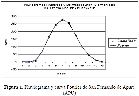
<p style="text-autospace: none" align="justify"><font face="Verdana"> <span style="font-family: TimesNewRoman"><font size="2">La intención es obtener  una cantidad de parámetros que sea menor al número de meses del año (12) para  que la solución sea </font></span><i> <span style="font-family: TimesNewRoman\,Italic"><font size="2">parsimoniosa</font></span></i><span style="font-family: TimesNewRoman"><font size="2">.  Se ha resaltado que los tres primeros armónicos explican al menos el 92% de la  variación total de la pluviosidad mensual, lo cual se consideró como una  representación Fourier pertinente para la función pluvial </font></span><i> <span style="font-family: TimesNewRoman\,Italic"><font size="2">f(t).</font></span></i></font></p>     <p style="text-autospace: none" align="justify"><font face="Verdana"> <span style="font-family: TimesNewRoman"><font size="2">Para evaluar el grado de  aproximación que se logra representando a </font></span><i> <span style="font-family: TimesNewRoman\,Italic"><font size="2">f (t) </font> </span></i><span style="font-family: TimesNewRoman"><font size="2">con los 3  primeros armónicos, se presentan, a modo de ejemplo, los gráficos de la serie  pluvial original de </font></span><i> <span style="font-family: TimesNewRoman\,Italic"><font size="2">San Fernando de  Apure </font></span></i><span style="font-family: TimesNewRoman"><font size="2"> y su representación </font></span><i> <span style="font-family: TimesNewRoman\,Italic"><font size="2">Fourier</font></span></i><span style="font-family: TimesNewRoman"><font size="2">,  modelo trigonométrico que explica el </font></span><i> <span style="font-family: TimesNewRoman\,Italic"><font size="2">99,83% </font> </span></i><span style="font-family: TimesNewRoman"><font size="2">de la  varianza total.</font></span></font></p>     <p style="text-autospace: none" align="center"> <img border="0" src="/img/fbpe/t/v26n39/art03fig1.gif" width="561" height="390"></p>     
<p style="text-autospace: none" align="justify"><font face="Verdana" size="2"> Apréciese que la serie Fourier de la sucesión pluvial reproduce bastante bien la  gráfica original, concluyéndose que los 6 parámetros Fourier serían suficientes  para analizar el régimen pluvial en el año.</font></p>     <p style="text-autospace: none" align="justify"><font face="Verdana" size="2"> Cada función armónica <i>f<sub>K</sub></i>(<i>t</i>) = <i>A<sub>K</sub></i> <i> cosk</i> <i>w</i><sub>0</sub><i>t</i> + <i>B<sub>K</sub></i> <i>senk</i> <i>w</i><sub>0</sub><i>t</i>  puede transformarse en una función trigonométrica cosenoidal o senoidal única.  Por ejemplo, se cumplirá que (H. P. Hsu; 1973; 5; J. Quinet; 1982; 159):</font></p>     <p style="text-autospace: none" align="center"> <img border="0" src="/img/fbpe/t/v26n39/art03ec15.gif" width="447" height="50"></p>     
<p style="text-autospace: none" align="justify"><font face="Verdana"> <span style="font-family: TimesNewRoman"><font size="2"><i>C<sub>K</sub></i> cos  (<i>k w</i><sub>0</sub><i>t</i> - </font><font face="Symbol"><font size="2">F</font></font><font size="2" face="Verdana"><i><sub>K</sub></i>)  representación </font></span><i> <span style="font-family: TimesNewRoman\,Italic"><font size="2">polar </font> </span></i><span style="font-family: TimesNewRoman"><font size="2">de la suma k-ésima  de Fourier</font></span></font></p>     <p style="text-autospace: none" align="justify"><font face="Verdana"> <span style="font-family: TimesNewRoman"><font size="2">C</font></span><sub><font size="2"><span style="font-family: TimesNewRoman">K</span></font></sub><span style="font-family: TimesNewRoman"><font size="2">a  amplitud del k-ésimo armónico</font></span></font></p>     ]]></body>
<body><![CDATA[<p style="text-autospace: none" align="justify"> <span style="font-family: TimesNewRoman"><font size="2" face="Verdana"><sub>K</sub>a </font> <font size="2" face="Symbol">º</font><font size="2" face="Verdana"> ángulo de fase, cosenoidal,  del k-ésimo armónico.</font></span></p>     <p align="justify"><font face="Verdana"> <span style="font-family: TimesNewRoman"><font size="2">Por ejemplo, para f<sub>1</sub>  (t), cuando T = 12 meses, es</font></span></font></p>     <p align="center"> <img border="0" src="/img/fbpe/t/v26n39/art03ec15a.gif" width="170" height="26"></p>     
<p style="text-autospace: none" align="justify"><font face="Verdana" size="2"> <span style="font-family: TimesNewRoman">Donde:</span></font></p>     <p style="text-autospace: none" align="justify"><font face="Verdana"> <span style="font-family: TimesNewRoman"><font size="2">C</font><sub><font size="2">1</font></sub><font size="2">  = amplitud –máximo valor de f</font><sub><font size="2">1</font></sub><font size="2">  (t)— del primer armónico</font></span></font></p>     <p style="text-autospace: none" align="justify"><font face="Verdana"> <span lang="FR" style="font-family: TimesNewRoman"><font size="2">W</font><sub><font size="2">0</font></sub><font size="2">  = 2 À / T = 2 À rad / 12 meses = 0,524 rad / mes a 30 ° / mes</font></span></font></p>     <p style="text-autospace: none" align="justify"><font face="Verdana"> <span style="font-family: TimesNewRoman"><font size="2">W</font></span><sub><span style="font-family: TimesNewRoman"><font size="2">0</font></span></sub><span style="font-family: TimesNewRoman"><font size="2">=  frecuencia fundamental</font></span></font></p>     <p style="text-autospace: none" align="justify"><font face="Verdana"> <span style="font-family: TimesNewRoman"><sub><font size="2">1</font></sub><font size="2">  = ángulo de fase cosenoidal del primer armónico</font></span></font></p>     <p style="text-autospace: none" align="justify"><font face="Verdana"> <span style="font-family: TimesNewRoman"><sub><font size="2">1</font></sub><font size="2">  = arc tg (B</font><sub><font size="2">1</font></sub><font size="2"> / A</font></span><sub><span style="font-family: TimesNewRoman"><font size="2">1</font></span></sub><span style="font-family: TimesNewRoman"><font size="2">)</font></span></font></p>     <p align="justify"><font face="Verdana" size="2"> <span style="font-family: TimesNewRoman">En el caso de la estación San Fernando  de Apure se tiene que</span></font></p>     ]]></body>
<body><![CDATA[<p align="center"> <img border="0" src="/img/fbpe/t/v26n39/art03ec16.gif" width="207" height="60"></p>     
<p align="justify"><font face="Verdana" size="2">Por lo tanto,</font></p>     <p align="center"> <img border="0" src="/img/fbpe/t/v26n39/art03ec16a.gif" width="398" height="31"></p>     
<p align="justify"><font face="Verdana" size="2">En cuanto al ángulo de fase  cosenoidal (AFC<sub>1</sub> = <sub>1</sub>), se obtiene</font></p>     <p align="center"> <img border="0" src="/img/fbpe/t/v26n39/art03ec16b.gif" width="334" height="55"></p>     
<p align="justify"><font face="Verdana" size="2">En consecuencia,</font></p>     <p align="center"> <img border="0" src="/img/fbpe/t/v26n39/art03ec16c.gif" width="395" height="49"></p>     
<p style="text-autospace: none" align="justify"><font face="Verdana"> <span style="font-family: TimesNewRoman"><font size="2">Para f</font><sub><font size="2">1</font></sub><font size="2">  (t), ello significa que su máximo valor C</font><sub><font size="2">1</font></sub><font size="2">  se halla a una distancia angular de </font></span><i> <span style="font-family: TimesNewRoman\,Italic"><font size="2">215,05º</font></span></i><span style="font-family: TimesNewRoman"><font size="2">.</font></span></font></p>     <p style="text-autospace: none" align="justify"><font face="Verdana" size="2">En  virtud de que la forma polar <i>f</i><sub><i>k</i></sub>(<i>t</i>) = <i>C<sub>k</sub></i>  cos(<i>kw</i><sub>0</sub><i>t</i> - </font><font size="2" face="Symbol">F</font><font face="Verdana" size="2"><i><sub>k</sub></i>)  es más adecuada que la forma binómica<i> f<sub>k</sub></i>(<i>t</i>) = <i>A<sub>k</sub></i>  cos<i>kw</i><sub>0</sub><i>t</i> + <i>B<sub>k</sub></i> sen<i>kw</i><sub>0</sub><i>t </i>porque incluye 2 de las características asociadas al comportamiento pluvial  en el régimen anual (máximo valor y localización de éste), se decidió elaborar  una base de datos de <i>15 x 6</i> valores, donde, ahora, los seis valores se  corresponden con las amplitudes y ángulos de fase cosenoidales de los tres  primeros armónicos.</font></p>     <p style="text-autospace: none" align="justify"><font face="Verdana" size="2"> Pero, debido a que la amplitud y el ángulo de fase se expresan en unidades  distintas, se creó una matriz estandarizada de datos, que se anexa de inmediato,  que hiciera posible la interpretación de los resultados del análisis  multivariable de agrupamiento que se aplicaría subsiguientemente.</font></p>     ]]></body>
<body><![CDATA[<p style="text-autospace: none" align="center"> <img border="0" src="/img/fbpe/t/v26n39/art03cua7.gif" width="574" height="358"></p>     
<p style="text-autospace: none" align="justify"><font face="Verdana"><b><i> <span style="font-family: TimesNewRoman\,BoldItalic"><font size="2"> DETERMINACIÓN DE LOS GRUPOS DE ESTACIONES PLUVIOMÉTRICAS CON IGUAL RÉGIMEN  PLUVIAL ANUAL</font></span></i></b></font></p>     <p style="text-autospace: none" align="justify"><font face="Verdana"> <span style="font-family: TimesNewRoman"><font size="2">Como se comentó en el  ítem anterior, se sustituyó la base de quince estaciones con sus doce valores  pluviales mensuales (</font></span><i><span style="font-family: TimesNewRoman\,Italic"><font size="2">15  x 12 = 180 </font></span></i><span style="font-family: TimesNewRoman"> <font size="2">datos) por una nueva base de datos constituidas por los  coeficientes Fourier estandarizados de los primeros 3 componentes armónicos, los  cuales explican, al menos, el 92% de la variación total de la pluviosidad  mensual de cada lugar; tal varianza explicada se consideró, tanto numérica como  climáticamente, que formaban una representación Fourier pertinente para la  función pluvial </font></span><i> <span style="font-family: TimesNewRoman\,Italic"><font size="2">f(t) </font> </span></i><span style="font-family: TimesNewRoman"><font size="2">respectiva.</font></span></font></p>     <p style="text-autospace: none" align="justify"><font face="Verdana" size="2"> <span style="font-family: TimesNewRoman">Seguidamente, se indagó acerca de  cuántos regímenes pluviales distintos estaban definidos por los quince casos  seleccionados. Para obtener la solución a tal propuesta se aplicó la siguiente  estrategia:</span></font></p>     <p style="text-autospace: none" align="justify"><font face="Verdana"> <span style="font-family: TimesNewRoman"><font size="2">1. Aplicación del  algoritmo del </font></span><i><span style="font-family: TimesNewRoman\,Italic"> <font size="2">promedio ponderado </font></span></i> <span style="font-family: TimesNewRoman"><font size="2">(Average Linkage, en  inglés) con distancia euclidiana con el propósito de evaluar qué cantidad de  grupos es la adecuada. El promedio ponderado (</font></span><i><span style="font-family: TimesNewRoman\,Italic"><font size="2">PP</font></span></i><span style="font-family: TimesNewRoman"><font size="2">)  es un algoritmo aglomerativo, jerárquico, combinatorial, compatible y  espacialmente invariante (véase, Propuesta de una Metodología de Clasificación  Climática Mediante la aplicación de Técnicas Multivariables a Indicadores  Geográficos-Ambientales; Marzo 2005; 208-223). El programa estadístico posee un  coeficiente llamado ÍNDICE DE SIMILITUD que orienta al usuario acerca del número  conveniente de grupos, el cual se complementa con el respectivo dendrograma. En  ese orden de ideas, se seleccionaron siete grupos.</font></span></font></p>     <p style="text-autospace: none" align="justify"><font face="Verdana"> <span style="font-family: TimesNewRoman"><font size="2">2. </font></span><i> <span style="font-family: TimesNewRoman\,Italic"><font size="2">Corrida </font> </span></i><span style="font-family: TimesNewRoman"><font size="2">del algoritmo  promedio ponderado, con distancia euclidiana, requiriéndosele que formara siete  grupos, los cuales quedaron constituidos de la forma siguiente:</font></span></font></p>     <p style="text-autospace: none" align="center"> <img border="0" src="/img/fbpe/t/v26n39/art03cua8.gif" width="313" height="206"></p>     
<p style="text-autospace: none" align="justify"><font face="Verdana" size="2"> <span style="font-family: TimesNewRoman">El cuadro señala, por ejemplo, que las  estaciones CORO (COR) y MAIQUETÍA (MIQ) tienen un régimen pluvial semejante,  según la base estandarizada de Fourier, de modo que constituyen el grupo cuatro.</span></font></p>     <p style="text-autospace: none" align="justify"><font face="Verdana"> <span style="font-family: TimesNewRoman"><font size="2">3. A fin de validar la  solución que genera el procedimiento </font></span><i> <span style="font-family: TimesNewRoman\,Italic"><font size="2">semiautomático </font></span></i><span style="font-family: TimesNewRoman"><font size="2"> anterior, se aplicaron otros algoritmos del programa estadístico, los cuales se  consideró no eran satisfactorios en relación con el promedio ponderado </font> </span><i><span style="font-family: TimesNewRoman\,Italic"><font size="2">(PP)</font></span></i><span style="font-family: TimesNewRoman"><font size="2">.  El dendrograma (<a href="#fig2">figura 2</a>) donde se muestran estos siete  grupos. La línea continua gruesa señala, de modo aproximado, los siete grupos  formados.</font></span></font></p>     <p style="text-autospace: none" align="center"><a name="fig2"> <img border="0" src="/img/fbpe/t/v26n39/art03fig2.gif" width="503" height="333"></a></p>     
]]></body>
<body><![CDATA[<p style="text-autospace: none" align="justify"><font face="Verdana"> <span style="font-family: TimesNewRoman"><font size="2">4. Las 6 variables  estandarizadas de las amplitudes y ángulos de fase cosenoidales forman un  sistema cartesiano oblicuo, lo que impide que la distancia euclidiana sea la  verdadera distancia de los casos en el espacio no métrico de las variables  citadas. En consecuencia, se </font></span><i> <span style="font-family: TimesNewRoman\,Italic"><font size="2">ortogonalizó </font></span></i><span style="font-family: TimesNewRoman"><font size="2">el  espacio </font></span><i><span style="font-family: TimesNewRoman\,Italic"> <font size="2">R6 </font></span></i><span style="font-family: TimesNewRoman"> <font size="2">de las variables mediante la técnica multivariable de Componentes  Principales (ACP) y luego se aplicó el algoritmo PP, resultando una solución no  pertinente cuando se utilizó como validación la gráfica pluvial de los datos  originales de los quince sitios.</font></span></font></p>     <p style="text-autospace: none" align="justify"><font face="Verdana" size="2">5.  Finalmente, se decidió que el algoritmo <i>PP</i> con distancia euclidiana era  el apropiado, aunque la distancia entre los casos podía estar sobre o  subestimada por una cantidad que depende del signo y magnitud de la correlación  o ángulo entre las variables.</font></p>     <p style="text-autospace: none" align="justify"><font face="Verdana" size="2"> <b>RESULTADOS</b></font></p>     <p style="text-autospace: none" align="justify"><font face="Verdana" size="2"> Para comprobar lo pertinente de la agrupación homogénea de regímenes pluviales  realizados mediante la metodología aplicada se presentan los distintos  pluviogramas para cada grupo especificado.</font></p>     <p style="text-autospace: none" align="center"> <img border="0" src="/img/fbpe/t/v26n39/art03gru1.gif" width="537" height="475"></p>     
<p style="text-autospace: none" align="center"> <img border="0" src="/img/fbpe/t/v26n39/art03gru2.gif" width="538" height="265"></p>     
<p style="text-autospace: none" align="center"> <img border="0" src="/img/fbpe/t/v26n39/art03gru3.gif" width="530" height="430"></p>     
<p style="text-autospace: none" align="center"> <img border="0" src="/img/fbpe/t/v26n39/art03gru4.gif" width="523" height="248"></p>     
<p style="text-autospace: none" align="center"> <img border="0" src="/img/fbpe/t/v26n39/art03gru5.gif" width="525" height="421"></p>     
<p style="text-autospace: none" align="justify"><font face="Verdana" size="2">El  programa <i>MINITAB</i> versión 13.2 produce una serie de estadísticas de las  características de los grupos formados, índices que se reproducen parcialmente.</font></p>     ]]></body>
<body><![CDATA[<p style="text-autospace: none" align="center"> <img border="0" src="/img/fbpe/t/v26n39/art03cua9.gif" width="534" height="251"></p>     
<p style="text-autospace: none" align="justify"><font face="Verdana" size="2">En  la columna 4 se compila la Distancia Promedio de los casos respecto al <i> centroide</i> del grupo (DPC), índice que permite cuantificar la homogeneidad  interna del grupo. De esta manera, se puede elaborar el <a href="#cua10">cuadro  10</a>.</font></p>     <p style="text-autospace: none" align="center"><a name="cua10"> <img border="0" src="/img/fbpe/t/v26n39/art03cua10.gif" width="527" height="212"></a></p>     
<p style="text-autospace: none" align="justify"><font face="Verdana" size="2">En  este cuadro se muestra que los grupos más homogéneos son los grupos 5, 6 y 7,  con un solo caso (Mérida, Puerto Ayacucho y San Antonio del Táchira,  respectivamente), mientras que el menos homogéneo es el grupo 1 (Barcelona,  Ciudad Bolívar, Maturín y San Fernando de Apure), ello significa que, en el  grupo 1 es donde hay menos semejanza en las amplitudes y ángulos de fase  cosenoidales estandarizados y por tanto, según nuestra hipótesis, en los  regímenes pluviales.</font></p>     <p style="text-autospace: none" align="justify"><font face="Verdana" size="2">Si  se desea £ escoger el caso más representativo en los grupos múltiples, <i> MINITAB</i> estima la distancia de cada estación con respecto al centroide del  grupo; de ahí que el caso con menor distancia al centroide puede escogerse como  el representante del grupo. En ese orden de ideas, se obtuvieron los siguientes  resultados:</font></p>     <p style="text-autospace: none" align="center"> <img border="0" src="/img/fbpe/t/v26n39/art03cua11.gif" width="524" height="239"></p>     
<p style="text-autospace: none" align="justify"><font face="Verdana" size="2"> Ciudad Bolívar (CBO) tiene la menor distancia al centroide del grupo 1 (véase  columna 3) lugar que tiene el siguiente pluviograma. Se trata de una curva  unimodal con máximo pluvial en julio. Colonia Tovar (COL) tiene la menor  distancia al centroide del grupo 3 (véase columna 3), sitio que tiene el  siguiente pluviograma. Se trata de una curva unimodal pero con leve descenso  antes de alcanzar su máximo pluvial en octubre. Dado que la distancia centroidal  de los casos es la misma, es indistinto escoger el caso representativo. Por  ejemplo, en Barquisimeto (BRQ) se aprecia una curva unimodal con un mínimo local  secundario pluvial en septiembre. La estación Coro (COR), exhibe una curva sin  estacionalidad anual pero con mínimo local secundario en agosto. Gráficamente se  tiene:</font></p>     <p style="text-autospace: none" align="center"> <img border="0" src="/img/fbpe/t/v26n39/art03gru11.gif" width="549" height="424"></p>     
<p style="text-autospace: none" align="justify"><font face="Verdana" size="2"> <b>CONCLUSIONES</b></font></p>     <p style="text-autospace: none" align="justify"><font face="Verdana" size="2">La  reducción de los doce montos pluviales, de un grupo seleccionado de quince  lugares, a seis coeficientes estandarizados de amplitudes y ángulos de fase  cosenoidales de las series Fourier, con aplicación a posteriori de un  procedimiento de agrupación automático supervisado, ha resultado ser apropiado  en cuanto a que ha permitido definir hasta 7 grupos de regímenes pluviales;  estos regímenes se distinguen por su estacionalidad anual (unimodal, bimodal, no  estacional), así como por la localización y magnitud de los valores pluviales  máximos y mínimos.</font></p>     ]]></body>
<body><![CDATA[<p style="text-autospace: none" align="justify"><font face="Verdana" size="2"> Esos resultados sugieren que la parametrización con las series Fourier es una  opción válida para caracterizar el régimen anual de la lluvia (así como de  cualquier otro elemento climático) e incorporarlos a una base de datos, tanto  por su enfoque reduccionista como por la posibilidad de obtener una mayor  discriminación del patrón de la distribución espacial que la lograda por los  procedimientos climáticos convencionales.</font></p>      <p style="text-autospace: none" align="justify"><font face="Verdana"><b> <span style="font-family: TimesNewRoman\,Bold"><font size="2">REFERENCIAS  BIBLIOGRÁFICAS</font></span></b></font></p>     <!-- ref --><p style="text-autospace: none" align="justify"><font face="Verdana"> <span style="font-family: TimesNewRoman"><font size="2">1. Cañada, A. (2002). </font></span><i><span style="font-family: TimesNewRoman\,Italic"> <font size="2">Series de Fourier y aplicaciones: Un tratado elemental con notas  históricas y ejercicios resueltos</font></span></i><span style="font-family: TimesNewRoman"><font size="2">. </font></span><span lang="EN-US" style="font-family: TimesNewRoman"> <font size="2">Ediciones Pirámide.</font></span></font>&nbsp;&nbsp;&nbsp;&nbsp;&nbsp;&nbsp;&nbsp;&nbsp;[&#160;<a href="javascript:void(0);" onclick="javascript: window.open('/scielo.php?script=sci_nlinks&ref=3315448&pid=S1012-7089201000010000300001&lng=','','width=640,height=500,resizable=yes,scrollbars=1,menubar=yes,');">Links</a>&#160;]<!-- end-ref --><!-- ref --><p style="text-autospace: none" align="justify"><font face="Verdana"> <span lang="EN-US" style="font-family: TimesNewRoman"><font size="2">2. Howell,  K.B. (2001). </font></span><i> <span lang="EN-US" style="font-family: TimesNewRoman\,Italic"><font size="2"> Principles of Fourier Analysis</font></span></i><span lang="EN-US" style="font-family: TimesNewRoman"><font size="2">.  Chapman &amp; Hall/CRC.</font></span></font>&nbsp;&nbsp;&nbsp;&nbsp;&nbsp;&nbsp;&nbsp;&nbsp;[&#160;<a href="javascript:void(0);" onclick="javascript: window.open('/scielo.php?script=sci_nlinks&ref=3315449&pid=S1012-7089201000010000300002&lng=','','width=640,height=500,resizable=yes,scrollbars=1,menubar=yes,');">Links</a>&#160;]<!-- end-ref --><!-- ref --><p style="text-autospace: none" align="justify"><font face="Verdana"> <span lang="EN-US" style="font-family: TimesNewRoman"><font size="2">3. Hsu, H.  P. (1973). </font></span><i><span style="font-family: TimesNewRoman\,Italic"> <font size="2">Análisis de Fourier</font></span></i><span style="font-family: TimesNewRoman"><font size="2">.  Fondo Educativo Interamericana. </font></span> <span lang="EN-US" style="font-family: TimesNewRoman"><font size="2">EEUU.</font></span></font>&nbsp;&nbsp;&nbsp;&nbsp;&nbsp;&nbsp;&nbsp;&nbsp;[&#160;<a href="javascript:void(0);" onclick="javascript: window.open('/scielo.php?script=sci_nlinks&ref=3315450&pid=S1012-7089201000010000300003&lng=','','width=640,height=500,resizable=yes,scrollbars=1,menubar=yes,');">Links</a>&#160;]<!-- end-ref --><!-- ref --><p style="text-autospace: none" align="justify"><font face="Verdana"> <span style="font-family: TimesNewRoman"><font size="2">4. Kyrkyla, K. I. y  Hameed, S. (1989). </font></span><i> <span lang="EN-US" style="font-family: TimesNewRoman\,Italic"><font size="2"> Harmonic analysis of the seasonal cycle in precipitation over the United Status:  a comparison between observations and a general circulation model</font></span></i><span lang="EN-US" style="font-family: TimesNewRoman"><font size="2">.  Journal of Climatology, 2 (12), 1463-1475.</font></span></font>&nbsp;&nbsp;&nbsp;&nbsp;&nbsp;&nbsp;&nbsp;&nbsp;[&#160;<a href="javascript:void(0);" onclick="javascript: window.open('/scielo.php?script=sci_nlinks&ref=3315451&pid=S1012-7089201000010000300004&lng=','','width=640,height=500,resizable=yes,scrollbars=1,menubar=yes,');">Links</a>&#160;]<!-- end-ref --><!-- ref --><p style="text-autospace: none" align="justify"><font face="Verdana"> <span lang="EN-US" style="font-family: TimesNewRoman"><font size="2">5. Quine,  J. T. (1982). </font></span><i> <span lang="PT-BR" style="font-family: TimesNewRoman\,Italic"><font size="2"> Curso de matemática superior</font></span></i><span lang="PT-BR" style="font-family: TimesNewRoman"><font size="2">.  Editorial Paraninfo. </font></span><span style="font-family: TimesNewRoman"> <font size="2">España.</font></span></font>&nbsp;&nbsp;&nbsp;&nbsp;&nbsp;&nbsp;&nbsp;&nbsp;[&#160;<a href="javascript:void(0);" onclick="javascript: window.open('/scielo.php?script=sci_nlinks&ref=3315452&pid=S1012-7089201000010000300005&lng=','','width=640,height=500,resizable=yes,scrollbars=1,menubar=yes,');">Links</a>&#160;]<!-- end-ref --><!-- ref --><p style="text-autospace: none" align="justify"><font face="Verdana" size="2"> <span style="font-family: TimesNewRoman">6. Programa estadístico MINITAB versión  13.2.</span></font>&nbsp;&nbsp;&nbsp;&nbsp;&nbsp;&nbsp;&nbsp;&nbsp;[&#160;<a href="javascript:void(0);" onclick="javascript: window.open('/scielo.php?script=sci_nlinks&ref=3315453&pid=S1012-7089201000010000300006&lng=','','width=640,height=500,resizable=yes,scrollbars=1,menubar=yes,');">Links</a>&#160;]<!-- end-ref --><!-- ref --><p style="text-autospace: none" align="justify"><font face="Verdana"> <span style="font-family: TimesNewRoman"><font size="2">7. Rodríguez G., J.  (1994). </font></span><i><span style="font-family: TimesNewRoman\,Italic"> <font size="2">Conceptos básicos el análisis armónico</font></span></i><span style="font-family: TimesNewRoman"><font size="2">.  Trabajo de ascenso a la categoría de asociado. UCV-Caracas.</font></span></font>&nbsp;&nbsp;&nbsp;&nbsp;&nbsp;&nbsp;&nbsp;&nbsp;[&#160;<a href="javascript:void(0);" onclick="javascript: window.open('/scielo.php?script=sci_nlinks&ref=3315454&pid=S1012-7089201000010000300007&lng=','','width=640,height=500,resizable=yes,scrollbars=1,menubar=yes,');">Links</a>&#160;]<!-- end-ref --><!-- ref --><p style="text-autospace: none" align="justify"><font face="Verdana"> <span style="font-family: TimesNewRoman"><font size="2">8. Rodríguez G., J.  (2003). </font></span><i><span style="font-family: TimesNewRoman\,Italic"> <font size="2">Distribución de las fechas del inicio de la temporada lluviosa  mediante análisis armónico de la región centro norte de Venezuela</font></span></i><span style="font-family: TimesNewRoman"><font size="2">.  Estudios Geográficos, LXIV (251), (335-346). Instituto de Economía y Geografía.  Madrid, España. Publicación trimestral.</font></span></font>&nbsp;&nbsp;&nbsp;&nbsp;&nbsp;&nbsp;&nbsp;&nbsp;[&#160;<a href="javascript:void(0);" onclick="javascript: window.open('/scielo.php?script=sci_nlinks&ref=3315455&pid=S1012-7089201000010000300008&lng=','','width=640,height=500,resizable=yes,scrollbars=1,menubar=yes,');">Links</a>&#160;]<!-- end-ref --><!-- ref --><p style="text-autospace: none" align="justify"><font face="Verdana"> <span style="font-family: TimesNewRoman"><font size="2">9. Rodríguez G., J.  (2005). </font></span><i><span style="font-family: TimesNewRoman\,Italic"> <font size="2">Propuesta de una metodología de una clasificación climática </font></span></i><span style="font-family: TimesNewRoman"><font size="2"> Trabajo de Especialización en Análisis de Datos en Ciencias Sociales. UCV-Caracas.</font></span></font>&nbsp;&nbsp;&nbsp;&nbsp;&nbsp;&nbsp;&nbsp;&nbsp;[&#160;<a href="javascript:void(0);" onclick="javascript: window.open('/scielo.php?script=sci_nlinks&ref=3315456&pid=S1012-7089201000010000300009&lng=','','width=640,height=500,resizable=yes,scrollbars=1,menubar=yes,');">Links</a>&#160;]<!-- end-ref --> ]]></body>
<back>
<ref-list>
<ref id="B1">
<label>1</label><nlm-citation citation-type="book">
<person-group person-group-type="author">
<name>
<surname><![CDATA[Cañada]]></surname>
<given-names><![CDATA[A]]></given-names>
</name>
</person-group>
<source><![CDATA[Series de Fourier y aplicaciones: Un tratado elemental con notas históricas y ejercicios resueltos]]></source>
<year>2002</year>
<publisher-name><![CDATA[Ediciones Pirámide]]></publisher-name>
</nlm-citation>
</ref>
<ref id="B2">
<label>2</label><nlm-citation citation-type="book">
<person-group person-group-type="author">
<name>
<surname><![CDATA[Howell]]></surname>
<given-names><![CDATA[K.B]]></given-names>
</name>
</person-group>
<source><![CDATA[Principles of Fourier Analysis]]></source>
<year>2001</year>
<publisher-name><![CDATA[Chapman & Hall/CRC]]></publisher-name>
</nlm-citation>
</ref>
<ref id="B3">
<label>3</label><nlm-citation citation-type="book">
<person-group person-group-type="author">
<name>
<surname><![CDATA[Hsu]]></surname>
<given-names><![CDATA[H. P]]></given-names>
</name>
</person-group>
<source><![CDATA[Análisis de Fourier]]></source>
<year>1973</year>
<publisher-name><![CDATA[Fondo Educativo Interamericana]]></publisher-name>
</nlm-citation>
</ref>
<ref id="B4">
<label>4</label><nlm-citation citation-type="journal">
<person-group person-group-type="author">
<name>
<surname><![CDATA[Kyrkyla]]></surname>
<given-names><![CDATA[K. I]]></given-names>
</name>
<name>
<surname><![CDATA[Hameed]]></surname>
<given-names><![CDATA[S]]></given-names>
</name>
</person-group>
<article-title xml:lang="en"><![CDATA[Harmonic analysis of the seasonal cycle in precipitation over the United Status: a comparison between observations and a general circulation model]]></article-title>
<source><![CDATA[Journal of Climatology]]></source>
<year>1989</year>
<volume>2</volume>
<numero>12</numero>
<issue>12</issue>
<page-range>1463-1475</page-range></nlm-citation>
</ref>
<ref id="B5">
<label>5</label><nlm-citation citation-type="book">
<person-group person-group-type="author">
<name>
<surname><![CDATA[Quine]]></surname>
<given-names><![CDATA[J. T]]></given-names>
</name>
</person-group>
<source><![CDATA[Curso de matemática superior]]></source>
<year>1982</year>
<publisher-name><![CDATA[Editorial Paraninfo]]></publisher-name>
</nlm-citation>
</ref>
<ref id="B6">
<label>6</label><nlm-citation citation-type="">
<source><![CDATA[Programa estadístico MINITAB versión 13.2]]></source>
<year></year>
</nlm-citation>
</ref>
<ref id="B7">
<label>7</label><nlm-citation citation-type="">
<person-group person-group-type="author">
<name>
<surname><![CDATA[Rodríguez G]]></surname>
<given-names><![CDATA[J]]></given-names>
</name>
</person-group>
<source><![CDATA[Conceptos básicos el análisis armónico]]></source>
<year>1994</year>
</nlm-citation>
</ref>
<ref id="B8">
<label>8</label><nlm-citation citation-type="journal">
<person-group person-group-type="author">
<name>
<surname><![CDATA[Rodríguez G]]></surname>
<given-names><![CDATA[J]]></given-names>
</name>
</person-group>
<article-title xml:lang="es"><![CDATA[Distribución de las fechas del inicio de la temporada lluviosa mediante análisis armónico de la región centro norte de Venezuela]]></article-title>
<source><![CDATA[Estudios Geográficos]]></source>
<year>2003</year>
<volume>LXIV</volume>
<numero>251</numero>
<issue>251</issue>
<page-range>335-346</page-range><publisher-loc><![CDATA[Madrid ]]></publisher-loc>
<publisher-name><![CDATA[Instituto de Economía y Geografía]]></publisher-name>
</nlm-citation>
</ref>
<ref id="B9">
<label>9</label><nlm-citation citation-type="">
<person-group person-group-type="author">
<name>
<surname><![CDATA[Rodríguez G]]></surname>
<given-names><![CDATA[J]]></given-names>
</name>
</person-group>
<source><![CDATA[Propuesta de una metodología de una clasificación climática]]></source>
<year>2005</year>
</nlm-citation>
</ref>
</ref-list>
</back>
</article>