<?xml version="1.0" encoding="ISO-8859-1"?><article xmlns:mml="http://www.w3.org/1998/Math/MathML" xmlns:xlink="http://www.w3.org/1999/xlink" xmlns:xsi="http://www.w3.org/2001/XMLSchema-instance">
<front>
<journal-meta>
<journal-id>1316-4821</journal-id>
<journal-title><![CDATA[Universidad, Ciencia y Tecnología]]></journal-title>
<abbrev-journal-title><![CDATA[uct]]></abbrev-journal-title>
<issn>1316-4821</issn>
<publisher>
<publisher-name><![CDATA[AutanaBooks S.A.S. Revista de la Universidad Experimental Politécnica Antonio José de Sucre, Vice Rectorado Puerto Ordaz, Venezuela, gestionada en Ecuador por AutanaBooks]]></publisher-name>
</publisher>
</journal-meta>
<article-meta>
<article-id>S1316-48212006000400008</article-id>
<title-group>
<article-title xml:lang="es"><![CDATA[Aplicaciones de la función de Lambert en electrónica]]></article-title>
<article-title xml:lang="en"><![CDATA[Applications of lambert’s function in electronics]]></article-title>
</title-group>
<contrib-group>
<contrib contrib-type="author">
<name>
<surname><![CDATA[García Sánchez]]></surname>
<given-names><![CDATA[Francisco J]]></given-names>
</name>
<xref ref-type="aff" rid="A01"/>
</contrib>
<contrib contrib-type="author">
<name>
<surname><![CDATA[Ortiz-Conde]]></surname>
<given-names><![CDATA[Adelmo]]></given-names>
</name>
<xref ref-type="aff" rid="A01"/>
</contrib>
<contrib contrib-type="author">
<name>
<surname><![CDATA[Malobabic]]></surname>
<given-names><![CDATA[Slavica]]></given-names>
</name>
<xref ref-type="aff" rid="A01"/>
</contrib>
</contrib-group>
<aff id="A01">
<institution><![CDATA[,Universidad Simón Bolívar Dpto. de Electrónica ]]></institution>
<addr-line><![CDATA[Caracas ]]></addr-line>
<country>Venezuela</country>
</aff>
<pub-date pub-type="pub">
<day>00</day>
<month>09</month>
<year>2006</year>
</pub-date>
<pub-date pub-type="epub">
<day>00</day>
<month>09</month>
<year>2006</year>
</pub-date>
<volume>10</volume>
<numero>40</numero>
<fpage>235</fpage>
<lpage>243</lpage>
<copyright-statement/>
<copyright-year/>
<self-uri xlink:href="http://ve.scielo.org/scielo.php?script=sci_arttext&amp;pid=S1316-48212006000400008&amp;lng=en&amp;nrm=iso"></self-uri><self-uri xlink:href="http://ve.scielo.org/scielo.php?script=sci_abstract&amp;pid=S1316-48212006000400008&amp;lng=en&amp;nrm=iso"></self-uri><self-uri xlink:href="http://ve.scielo.org/scielo.php?script=sci_pdf&amp;pid=S1316-48212006000400008&amp;lng=en&amp;nrm=iso"></self-uri><abstract abstract-type="short" xml:lang="es"><p><![CDATA[Se presenta una revisión del uso de la función de Lambert en aplicaciones de electrónica. Primeramente se describe brevemente su definición y se mencionan algunas de sus propiedades. Seguidamente se ofrecen ejemplos de cómo aplicar esta función en la solución de algunas ecuaciones transcendentales que involucran exponenciales. Las aplicaciones de esta función a la electrónica se ilustran mediante ejemplos relativos a la solución de problemas de dispositivos bipolares de juntura, modelado de celdas solares bajo iluminación, y modelos de dispositivos MOSFET.]]></p></abstract>
<abstract abstract-type="short" xml:lang="en"><p><![CDATA[A revision of the use of Lambert’s function in electronics applications is presented. Firstly, its definition is briefly described and some of its properties are mentioned. Next, examples are worked out of how to apply this function to the solution of some transcendental equations which contain exponentials. Applications of this function to electronics are illustrated through examples dealing with the solution of problems such as bipolar junction devices, modelling of illuminated solar cells, and MOSFET device modelling]]></p></abstract>
<kwd-group>
<kwd lng="es"><![CDATA[Función de Lambert]]></kwd>
<kwd lng="es"><![CDATA[Junturas no ideales]]></kwd>
<kwd lng="es"><![CDATA[Celdas solares]]></kwd>
<kwd lng="es"><![CDATA[MOSFETs sin dopaje]]></kwd>
<kwd lng="en"><![CDATA[Lambert Function]]></kwd>
<kwd lng="en"><![CDATA[Non Ideal Junctions]]></kwd>
<kwd lng="en"><![CDATA[Solar Cells]]></kwd>
<kwd lng="en"><![CDATA[Undoped MOSFETs]]></kwd>
</kwd-group>
</article-meta>
</front><body><![CDATA[ <p ALIGN="center" style="word-spacing: 0; line-height: 100%"><span style="mso-fareast-font-family: Times New Roman; mso-ansi-language: ES; mso-fareast-language: ES; mso-bidi-language: AR-SA"><b><span style="mso-fareast-font-family: Times New Roman; mso-bidi-font-family: Times New Roman; mso-ansi-language: ES; mso-fareast-language: ES; mso-bidi-language: AR-SA"><font face="Verdana" size="3">Aplicaciones de la función de Lambert en</font></span></b> <font face="Verdana" size="3"> <b><span style="mso-fareast-font-family: Times New Roman; mso-bidi-font-family: Times New Roman; mso-ansi-language: ES; mso-fareast-language: ES; mso-bidi-language: AR-SA">electrónica</span></b></font></span></p>     <p ALIGN="center" style="word-spacing: 0; line-height: 100%"><font face="Verdana" size="2"><b>García Sánchez, Francisco J. Ortiz-Conde, Adelmo</b> </font><b><font face="Verdana" size="2">Malobabic, Slavica</font></p> </b>     <p ALIGN="justify" style="word-spacing: 0; line-height: 100%"><font size="2" face="Verdana">Los autores desempeñan sus actividades en el Dpto. de Electrónica de la Universidad Simón Bolívar, Apartado Postal 89000, Caracas 1080, Venezuela, telef-58-212-9064010, fax 58-212-9064025.</font></p>     <p ALIGN="justify" style="word-spacing: 0; line-height: 100%"><font size="2" face="Verdana">Dres. Francisco J. García Sánchez y Adelmo Ortiz-Conde: Profesores Titulares, correos electrónicos fgarcia@ieee.org y ortizc@ieee.org respectivamente.</font></p>     <p ALIGN="justify" style="word-spacing: 0; line-height: 100%"><font size="2" face="Verdana">Ing. Slavica Malobabic: Estudiante de Maestría, correo electrónico smalobabic@gmail.com.</font></p> <b>     <p ALIGN="justify" style="word-spacing: 0; line-height: 100%"><font size="2" face="Verdana">Resumen</font></b></p>     <p ALIGN="justify" style="word-spacing: 0; line-height: 100%"><font size="2" face="Verdana">Se presenta una revisión del uso de la función de Lambert en aplicaciones de electrónica. Primeramente se describe brevemente su definición y se mencionan algunas de sus propiedades. Seguidamente se ofrecen ejemplos de cómo aplicar esta función en la solución de algunas ecuaciones transcendentales que involucran exponenciales. Las aplicaciones de esta función a la electrónica se ilustran mediante ejemplos relativos a la solución de problemas de dispositivos bipolares de juntura, modelado de celdas solares bajo iluminación, y modelos de dispositivos MOSFET.</font></p> <b>     <p ALIGN="justify" style="word-spacing: 0; line-height: 100%"><font face="Verdana" size="2">Palabras clave: </font></b><font face="Verdana" size="2">Función de Lambert/ Junturas no ideales/ Celdas solares/ MOSFETs sin dopaje.</font></p>     <p ALIGN="center" style="word-spacing: 0; line-height: 100%"><font face="Verdana" size="2"><b><span lang="EN-US" style="mso-fareast-font-family: Times New Roman; mso-bidi-font-family: Times New Roman; mso-ansi-language: EN-US; mso-fareast-language: ES; mso-bidi-language: AR-SA">Applications of lambert’s</span></b><span lang="EN-US" style="mso-fareast-font-family: Times New Roman; mso-ansi-language: EN-US; mso-fareast-language: ES; mso-bidi-language: AR-SA"> </span><b><span lang="EN-US" style="mso-fareast-font-family: Times New Roman; mso-bidi-font-family: Times New Roman; mso-ansi-language: EN-US; mso-fareast-language: ES; mso-bidi-language: AR-SA">function in electronics</span></b></font></p>     <p ALIGN="justify" style="word-spacing: 0; line-height: 100%"><b><font size="2" face="Verdana">Abstract</font></b></p>     ]]></body>
<body><![CDATA[<p ALIGN="justify" style="word-spacing: 0; line-height: 100%"><font size="2" face="Verdana">A revision of the use of Lambert’s function in electronics applications is presented. Firstly, its definition is briefly described and some of its properties are mentioned. Next, examples are worked out of how to apply this function to the solution of some transcendental equations which contain exponentials. Applications of this function to electronics are illustrated through examples dealing with the solution of problems such as bipolar junction devices, modelling of illuminated solar cells, and MOSFET device modelling.</font></p> <b>     <p ALIGN="justify" style="word-spacing: 0; line-height: 100%"><font face="Verdana" size="2">Keywords: </font></b><font face="Verdana" size="2">Lambert Function/ Non Ideal Junctions/ Solar Cells/ Undoped MOSFETs.</font></p>     <p ALIGN="justify" style="word-spacing: 0; line-height: 100%"><font face="Verdana" size="2"><b>Finalizado</b>: 11/01/2006 <b>Recibido</b>: 23/02/2006 <b>Aceptado</b>: 13/06/2006</font></p> <b>     <p ALIGN="justify" style="word-spacing: 0; line-height: 100%"><font size="2" face="Verdana">I. INTRODUCCIÓN.</font></p> </b>     <p ALIGN="justify" style="word-spacing: 0; line-height: 100%"><font face="Verdana" size="2">Una gran variedad de problemas en la ciencia y la tecnología están descritos por ecuaciones transcendentales que requieren ya sea de soluciones numéricas iterativas o bien de soluciones analíticas aproximadas. La posibilidad de obtener soluciones analíticas exactas de estas ecuaciones ofrece grandes ventajas desde varios puntos de vista. Una solución analítica describe el comportamiento de la variable de forma general, a diferencia de los resultados numéricos que dependen de las condiciones iniciales. La solución analítica ayuda en el entendimiento intuitivo del problema, facilita la deducción de su comportamiento cuando los parámetros del problema varían, y simplifica el estudio de las perturbaciones. También puede contribuir en la unificación de fenómenos diferentes, y hace que el fenómeno en sí sea más manejable y fácil de entender. En general una solución analítica se puede diferenciar e integrar analíticamente, lo que permite estudiar la variabilidad del fenómeno.</font></p>     <p ALIGN="justify" style="word-spacing: 0; line-height: 100%"><font size="2" face="Verdana">Aunque ciertamente las soluciones numéricas iterativas pueden proveer soluciones tan exactas como se requiera, la solución analítica, por no presentar problemas de convergencia, produce resultados exactos de manera computacionalmente eficiente. Al eliminar la necesidad de iteraciones numéricas, la solución analítica posibilita la evaluación rápida de numerosos casos repetitivos, lo que es de fundamental importancia en situaciones de simulación circuital, donde un modelo se ha de utilizar miles, si no millones, de veces. Aún en los casos en que se decida utilizar iteración numérica, las soluciones analíticas pueden ser útiles para proveer valores iniciales de las soluciones, facilitando así los cálculos iterativos complicados, dependientes del tiempo o multidimensionales.</font></p>     <p ALIGN="justify" style="word-spacing: 0; line-height: 100%"><font face="Verdana" size="2">Existe una clase de ecuaciones transcendentales, las del tipo lineal exponencial, que son muy comunes en ciertos circuitos electrónicos y en el modelado de dispositivos semiconductores. La función de Lambert (W) [1] permite obtener soluciones cerradas y explícitas a estas ecuaciones transcendentales [2,3]. En este trabajo se presentará una revisión de la utilidad de la función de Lambert, empezando por una breve descripción de sus propiedades, seguida de algunos ejemplos de soluciones a ecuaciones transcendentales, así como aplicaciones típicas a problemas de electrónica. Las aplicaciones de esta función a la electrónica se ilustran mediante ejemplos relativos a la solución de problemas de junturas no ideales con resistencias parásitas en serie y en shunt, características corriente voltaje de dispositivos fotovoltaicos bajo iluminación, y modelos de dispositivos MOSFET.</font></p> <b>     <p ALIGN="justify" style="word-spacing: 0; line-height: 100%"><font size="2" face="Verdana">I. DESARROLLO</font></p>     <p ALIGN="justify" style="word-spacing: 0; line-height: 100%"><font size="2" face="Verdana">1. La función de Lambert</font></p> </b>     <p ALIGN="justify" style="word-spacing: 0; line-height: 100%"><font face="Verdana" size="2">La función de Lambert tiene sus orígenes en el trabajo de J. Lambert en el año 1758. Más tarde, en 1779, fue considerada por Euler cuando estudió la ecuación trascendental de Lambert. Fue denominada “W” después del trabajo hecho por E. M. Wright en 1959 [4]. Desde entonces ha venido siendo utilizada esporádicamente en algunas aplicaciones, pero en años recientes la cantidad y diversidad de aplicaciones en las que se ha usado esta función ha ido incrementándose considerablemente. Hasta la fecha se ha usado W en aplicaciones generales tales como ciertos problemas de física [5], electromagnetismo [6], mecánica estadística clásica [7], movimiento de proyectiles [8], generación de ruido gausiano [9,10], solución de exponenciales infinitos [11], solución de la ecuación de Schrödinger [12], etc. En el área de la electrónica se ha empleado W en resolver problemas de diodos con resistencias en serie y en paralelo [13,14], circuitos con transistores bipolares [15], celdas solares [16-18], modelado del fenómeno de ruptura en óxidos delgados [19], diseño de consumo mínimo en circuitos [20], y modelado de transistores de efecto de campo metal-óxido-semiconductor (MOSFETs) [21-26].</font></p>     ]]></body>
<body><![CDATA[<p ALIGN="justify" style="word-spacing: 0; line-height: 100%"><font size="2" face="Verdana">La función de Lambert es una función elementalmente implícita, es decir, está definida de forma implícita usando funciones elementales. Formalmente W se define para cualquier z compleja como una función (compleja y de valores múltiples) que es la solución a la ecuación trascendental quizás más simple que exista, la ecuación lineal exponencial, representada por:</font></p>     <p ALIGN="center" style="word-spacing: 0; line-height: 100%"><font face="Verdana" size="2"><img border="0" src="/img/fbpe/uct/v10n40/art08ecu1.jpg" width="380" height="72"></font></p>     
<p ALIGN="justify" style="word-spacing: 0; line-height: 100%"><font face="Verdana" size="2">En la <b><a href="#fig1"> Figura 1.a</a></b> se muestra z como el producto de W(z) por el exponencial de W(z) en función de W(z). Intercambiando los ejes se obtiene la función de Lambert W(z) en función de z que se muestra en la <a href="#fig1"><b> figura 1.b</b></a>. Para argumentos reales x, W(x) es real si x<span style="mso-fareast-font-family: Times New Roman; mso-ansi-language: ES; mso-fareast-language: ES; mso-bidi-language: AR-SA">&#8805;</span>-e<sup>-1</sup>. Usando la definición de la función de Lambert x=W(x)e<sup>W(x)</sup> se puede decir que si x=ye<sup>y</sup>, entonces W(x)=y, o lo que es lo mismo,</font></p>     <p ALIGN="center" style="word-spacing: 0; line-height: 100%"><font face="Verdana" size="2"><img border="0" src="/img/fbpe/uct/v10n40/art08ecu2.jpg" width="366" height="54"></font></p>     
<p ALIGN="justify" style="word-spacing: 0; line-height: 100%"><font size="2" face="Verdana">Observando la <b><a href="#fig1"> Figura 1.b</a></b> se puede ver que para valores del argumento x&lt;0 existen o bien dos soluciones (-e<sup>-1</sup><span style="mso-fareast-font-family: Times New Roman; mso-ansi-language: ES; mso-fareast-language: ES; mso-bidi-language: AR-SA">&#8805;x&gt;0</span>) o ninguna (x&lt;-e<sup>-1</sup>). Para valores reales de W los valores del argumento están limitados a . W tiene dos ramas reales: la rama principal y la rama negativa [27]. La rama principal W<sub>0</sub> está definida como:</font></p>     <p ALIGN="center" style="word-spacing: 0; line-height: 100%"><font face="Verdana" size="2"><img border="0" src="/img/fbpe/uct/v10n40/art08ecu3.jpg" width="399" height="40"></font></p>     
<p ALIGN="justify" style="word-spacing: 0; line-height: 100%"><font size="2" face="Verdana">y la rama negativa W-1 está definida como:</font></p>     <p ALIGN="center" style="word-spacing: 0; line-height: 100%"><font face="Verdana" size="2"><img border="0" src="/img/fbpe/uct/v10n40/art08ecu4.jpg" width="325" height="52"></font></p>     
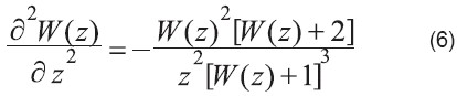
<p ALIGN="justify" style="word-spacing: 0; line-height: 100%"><font size="2" face="Verdana">Una de las características que hace atractivo el uso de expresiones basadas en la función de Lambert es que es analíticamente diferenciable e integrable. La primera y segunda derivadas están dadas por</font></p>     <p ALIGN="center" style="word-spacing: 0; line-height: 100%"><font face="Verdana" size="2"><img border="0" src="/img/fbpe/uct/v10n40/art08ecu5.jpg" width="404" height="73"></font></p>     
]]></body>
<body><![CDATA[<p ALIGN="center" style="word-spacing: 0; line-height: 100%"><font face="Verdana" size="2"><img border="0" src="/img/fbpe/uct/v10n40/art08ecu6.jpg" width="414" height="87"></font></p>     
<p ALIGN="left" style="word-spacing: 0; line-height: 100%"><a name="fig1"></a></p>     <p ALIGN="center" style="word-spacing: 0; line-height: 100%"><font face="Verdana" size="2"><img border="0" src="/img/fbpe/uct/v10n40/art08fig1.jpg" width="500" height="842"></font></p> <b>     
<p ALIGN="center" style="word-spacing: 0; line-height: 100%"><font face="Verdana" size="2">Figura 1. (a) z = W exp(W) en función de W (línea continua),</font></b><font size="2" face="Verdana"> <b>mostrando también las funciones exp(W) y W (líneas</b> <b>quebradas), (b) W en función de z, mostrando la rama</b>  </font><b><font face="Verdana" size="2">principal (línea continua) y la rama negativa (línea quebrada).</font></p> </b>     <p ALIGN="justify" style="word-spacing: 0; line-height: 100%"><font size="2" face="Verdana">La integral indefinida de la función de Lambert es</font></p>     <p ALIGN="center" style="word-spacing: 0; line-height: 100%"><font face="Verdana" size="2"><img border="0" src="/img/fbpe/uct/v10n40/art08ecu7.jpg" width="487" height="80"></font></p>     
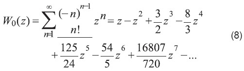
<p ALIGN="justify" style="word-spacing: 0; line-height: 100%"><font size="2" face="Verdana">La función de Lambert se puede representar mediante expansiones en series [28]. Por ejemplo la serie alrededor de z=0 es:</font></p>     <p ALIGN="center" style="word-spacing: 0; line-height: 100%"><font face="Verdana" size="2"><img border="0" src="/img/fbpe/uct/v10n40/art08ecu8.jpg" width="502" height="147"></font></p>     
<p ALIGN="justify" style="word-spacing: 0; line-height: 100%"><font size="2" face="Verdana">Igualmente existen representaciones asintóticas de W. La asíntota para z grande es</font></p>     <p ALIGN="center" style="word-spacing: 0; line-height: 100%"><font face="Verdana" size="2"><img border="0" src="/img/fbpe/uct/v10n40/art08ecu9.jpg" width="496" height="47"></font></p>     
]]></body>
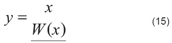
<body><![CDATA[<p ALIGN="justify" style="word-spacing: 0; line-height: 100%"><font size="2" face="Verdana">Existe disponible software numérico libre bien comprobado, con precisión numérica arbitraria, para las dos ramas reales de W. Por ejemplo, el Algoritmo 443 publicado en 1973 [29]. Más recientemente, en 1995, se publicó también el Algoritmo 743 de la base de datos TOMS de la librería pública Netlib ( software, escrito en FORTRAN, computa ambas ramas reales de W con la precisión disponible en la plataforma utilizada [31]. También existen aproximaciones eficientes [32]. Varios paquetes matemáticos simbólicos tales como: Maple®, Macsyma® y Mathematica® contienen rutinas optimizadas para el cálculo y manipulación de la función de Lambert, incluyendo su integración y diferenciación. En el paquete Mathematica®. la función de Lambert se denomina con el nombre de función “ProdutLog”. Varias aproximaciones incorporan esquemas iterativos para computar W con una precisión predefinida y usan aproximaciones a tramos para generar suposiciones iniciales [33].</font></p> <b>     <p ALIGN="justify" style="word-spacing: 0; line-height: 100%"><font size="2" face="Verdana">2. Ejemplos de soluciones usando W</font></p> </b>     <p ALIGN="justify" style="word-spacing: 0; line-height: 100%"><font size="2" face="Verdana">A continuación se presentaran algunos ejemplos que ilustran el procedimiento para resolver ecuaciones que contienen productos y cocientes de variables y sus exponenciales o logaritmos. No pretende esto ser una descripción exhaustiva de todos los casos en los que es posible usar W, sino que la intención es indicar la mecánica general del procedimiento a seguir.</font></p> <b>     <p ALIGN="justify" style="word-spacing: 0; line-height: 100%"><font size="2" face="Verdana">Ejemplo 1</font></p> </b>     <p ALIGN="justify" style="word-spacing: 0; line-height: 100%"><font size="2" face="Verdana">Ecuación:</font></p>     <p ALIGN="center" style="word-spacing: 0; line-height: 100%"><font face="Verdana" size="2"><img border="0" src="/img/fbpe/uct/v10n40/art08ecu10.jpg" width="361" height="39"></font></p>     
<p ALIGN="justify" style="word-spacing: 0; line-height: 100%"><font size="2" face="Verdana">Rescribir la ecuación (15) tomado exponenciales:</font></p>     <p ALIGN="center" style="word-spacing: 0; line-height: 100%"><font face="Verdana" size="2"><img border="0" src="/img/fbpe/uct/v10n40/art08ecu11.jpg" width="365" height="66"></font></p>     
<p ALIGN="justify" style="word-spacing: 0; line-height: 100%"><font size="2" face="Verdana">Multiplicar por x:</font></p>     <p ALIGN="center" style="word-spacing: 0; line-height: 100%"><font face="Verdana" size="2"><img border="0" src="/img/fbpe/uct/v10n40/art08ecu12.jpg" width="349" height="57"></font></p>     
]]></body>
<body><![CDATA[<p ALIGN="justify" style="word-spacing: 0; line-height: 100%"><font size="2" face="Verdana">Aplicar W a ambos lados:</font></p>     <p ALIGN="center" style="word-spacing: 0; line-height: 100%"><font face="Verdana" size="2"><img border="0" src="/img/fbpe/uct/v10n40/art08ecu13.jpg" width="376" height="55"></font></p>     
<p ALIGN="justify" style="word-spacing: 0; line-height: 100%"><font size="2" face="Verdana">Usar definición de W en la parte izquierda:</font></p>     <p ALIGN="center" style="word-spacing: 0; line-height: 100%"><font face="Verdana" size="2"><img border="0" src="/img/fbpe/uct/v10n40/art08ecu14.jpg" width="386" height="59"></font></p>     
<p ALIGN="justify" style="word-spacing: 0; line-height: 100%"><font size="2" face="Verdana">Solución:</font></p>     <p ALIGN="center" style="word-spacing: 0; line-height: 100%"><font face="Verdana" size="2"><img border="0" src="/img/fbpe/uct/v10n40/art08ecu15.jpg" width="350" height="89"></font></p> <b>     
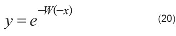
<p ALIGN="justify" style="word-spacing: 0; line-height: 100%"><font size="2" face="Verdana">Ejemplo 2</font></p> </b>     <p ALIGN="justify" style="word-spacing: 0; line-height: 100%"><font size="2" face="Verdana">Ecuación:</font></p>     <p ALIGN="center" style="word-spacing: 0; line-height: 100%"><font face="Verdana" size="2"><img border="0" src="/img/fbpe/uct/v10n40/art08ecu16.jpg" width="381" height="40"></font></p>     
<p ALIGN="justify" style="word-spacing: 0; line-height: 100%"><font size="2" face="Verdana">Rescribir la ecuación (16):</font></p>     ]]></body>
<body><![CDATA[<p ALIGN="center" style="word-spacing: 0; line-height: 100%"><font face="Verdana" size="2"><img border="0" src="/img/fbpe/uct/v10n40/art08ecu17.jpg" width="387" height="66"></font></p>     
<p ALIGN="justify" style="word-spacing: 0; line-height: 100%"><font size="2" face="Verdana">Aplicar W a ambos lados:</font></p>     <p ALIGN="center" style="word-spacing: 0; line-height: 100%"><font face="Verdana" size="2"><img border="0" src="/img/fbpe/uct/v10n40/art08ecu18.jpg" width="387" height="48"></font></p>     
<p ALIGN="justify" style="word-spacing: 0; line-height: 100%"><font size="2" face="Verdana">Usar definición de W en la parte derecha:</font></p>     <p ALIGN="center" style="word-spacing: 0; line-height: 100%"><font face="Verdana" size="2"><img border="0" src="/img/fbpe/uct/v10n40/art08ecu19.jpg" width="389" height="52"></font></p>     
<p ALIGN="justify" style="word-spacing: 0; line-height: 100%"><font size="2" face="Verdana">Solución:</font></p>     <p ALIGN="center" style="word-spacing: 0; line-height: 100%"><font face="Verdana" size="2"><img border="0" src="/img/fbpe/uct/v10n40/art08ecu20.jpg" width="358" height="74"></font></p> <b>     
<p ALIGN="justify" style="word-spacing: 0; line-height: 100%"><font size="2" face="Verdana">Ejemplo 3</font></p> </b>     <p ALIGN="justify" style="word-spacing: 0; line-height: 100%"><font size="2" face="Verdana">Ecuación:</font></p>     <p ALIGN="center" style="word-spacing: 0; line-height: 100%"><font face="Verdana" size="2"><img border="0" src="/img/fbpe/uct/v10n40/art08ecu21.jpg" width="354" height="44"></font></p>     
]]></body>
<body><![CDATA[<p ALIGN="justify" style="word-spacing: 0; line-height: 100%"><font size="2" face="Verdana">Rescribir la ecuación (21):</font></p>     <p ALIGN="center" style="word-spacing: 0; line-height: 100%"><font face="Verdana" size="2"><img border="0" src="/img/fbpe/uct/v10n40/art08ecu22.jpg" width="322" height="53"></font></p>     
<p ALIGN="justify" style="word-spacing: 0; line-height: 100%"><font size="2" face="Verdana">Aplicar a W a ambos lados:</font></p>     <p ALIGN="center" style="word-spacing: 0; line-height: 100%"><font face="Verdana" size="2"><img border="0" src="/img/fbpe/uct/v10n40/art08ecu23.jpg" width="335" height="52"></font></p>     
<p ALIGN="justify" style="word-spacing: 0; line-height: 100%"><font size="2" face="Verdana">Usar definición de W en la parte izquierda:</font></p>     <p ALIGN="center" style="word-spacing: 0; line-height: 100%"><font face="Verdana" size="2"><img border="0" src="/img/fbpe/uct/v10n40/art08ecu24.jpg" width="320" height="53"></font></p>     
<p ALIGN="justify" style="word-spacing: 0; line-height: 100%"><font size="2" face="Verdana">Solución:</font></p>     <p ALIGN="center" style="word-spacing: 0; line-height: 100%"><font face="Verdana" size="2"><img border="0" src="/img/fbpe/uct/v10n40/art08ecu25.jpg" width="332" height="49"></font></p> <b>     
<p ALIGN="justify" style="word-spacing: 0; line-height: 100%"><font size="2" face="Verdana">La función de Wright</font></p> </b>     <p ALIGN="justify" style="word-spacing: 0; line-height: 100%"><font size="2" face="Verdana">Se define como función de Wright [4,34] la solución a la ecuación (21), que se representa como</font></p>     ]]></body>
<body><![CDATA[<p ALIGN="center" style="word-spacing: 0; line-height: 100%"><font face="Verdana" size="2"><img border="0" src="/img/fbpe/uct/v10n40/art08ecu26.jpg" width="332" height="44"></font></p>     
<p ALIGN="justify" style="word-spacing: 0; line-height: 100%"><font size="2" face="Verdana">donde <span style="mso-fareast-font-family: Times New Roman; mso-ansi-language: ES; mso-fareast-language: ES; mso-bidi-language: AR-SA">&#969;</span> (omega) es la función de Wright. Comparando las ecuaciones (25) y (26) se puede establecer la equivalencia entre la función de Wright y la función de Lambert:</font></p> <b>     <p ALIGN="center" style="word-spacing: 0; line-height: 100%"><font face="Verdana" size="2"><img border="0" src="/img/fbpe/uct/v10n40/art08ecu27.jpg" width="335" height="55"></font></p>     
<p ALIGN="justify" style="word-spacing: 0; line-height: 100%"><font size="2" face="Verdana">Ejemplo 4</font></p> </b>     <p ALIGN="justify" style="word-spacing: 0; line-height: 100%"><font size="2" face="Verdana">Ecuación:</font></p>     <p ALIGN="center" style="word-spacing: 0; line-height: 100%"><font face="Verdana" size="2"><img border="0" src="/img/fbpe/uct/v10n40/art08ecu28.jpg" width="335" height="53"></font></p>     
<p ALIGN="justify" style="word-spacing: 0; line-height: 100%"><font size="2" face="Verdana">Primer procedimiento:</font></p>     <p ALIGN="justify" style="word-spacing: 0; line-height: 100%"><font size="2" face="Verdana">Rescribir la ecuación (28):</font></p>     <p ALIGN="center" style="word-spacing: 0; line-height: 100%"><font face="Verdana" size="2"><img border="0" src="/img/fbpe/uct/v10n40/art08ecu29.jpg" width="338" height="54"></font></p>     
<p ALIGN="justify" style="word-spacing: 0; line-height: 100%"><font size="2" face="Verdana">Aplicar W a ambos lados:</font></p>     ]]></body>
<body><![CDATA[<p ALIGN="center" style="word-spacing: 0; line-height: 100%"><font face="Verdana" size="2"><img border="0" src="/img/fbpe/uct/v10n40/art08ecu30.jpg" width="363" height="56"></font></p>     
<p ALIGN="justify" style="word-spacing: 0; line-height: 100%"><font size="2" face="Verdana">Usar definición de W en la parte izquierda:</font></p>     <p ALIGN="center" style="word-spacing: 0; line-height: 100%"><font face="Verdana" size="2"><img border="0" src="/img/fbpe/uct/v10n40/art08ecu31.jpg" width="352" height="74"></font></p>     
<p ALIGN="justify" style="word-spacing: 0; line-height: 100%"><font size="2" face="Verdana">Solución:</font></p>     <p ALIGN="center" style="word-spacing: 0; line-height: 100%"><font face="Verdana" size="2"><img border="0" src="/img/fbpe/uct/v10n40/art08ecu32.jpg" width="357" height="43"></font></p>     
<p ALIGN="justify" style="word-spacing: 0; line-height: 100%"><font size="2" face="Verdana">Segundo procedimiento:</font></p>     <p ALIGN="justify" style="word-spacing: 0; line-height: 100%"><font size="2" face="Verdana">Rescribir la ecuación (28):</font></p>     <p ALIGN="center" style="word-spacing: 0; line-height: 100%"><font face="Verdana" size="2"><img border="0" src="/img/fbpe/uct/v10n40/art08ecu33.jpg" width="358" height="51"></font></p>     
<p ALIGN="justify" style="word-spacing: 0; line-height: 100%"><font size="2" face="Verdana">Reagrupar:</font></p>     <p ALIGN="center" style="word-spacing: 0; line-height: 100%"><font face="Verdana" size="2"><img border="0" src="/img/fbpe/uct/v10n40/art08ecu34.jpg" width="360" height="59"></font></p>     
]]></body>
<body><![CDATA[<p ALIGN="justify" style="word-spacing: 0; line-height: 100%"><font size="2" face="Verdana">Aplicar W a ambos lados:</font></p>     <p ALIGN="center" style="word-spacing: 0; line-height: 100%"><font face="Verdana" size="2"><img border="0" src="/img/fbpe/uct/v10n40/art08ecu35.jpg" width="376" height="46"></font></p>     
<p ALIGN="justify" style="word-spacing: 0; line-height: 100%"><font size="2" face="Verdana">Usar definición de W en la parte derecha:</font></p>     <p ALIGN="center" style="word-spacing: 0; line-height: 100%"><font face="Verdana" size="2"><img border="0" src="/img/fbpe/uct/v10n40/art08ecu36.jpg" width="386" height="56"></font></p>     
<p ALIGN="justify" style="word-spacing: 0; line-height: 100%"><font size="2" face="Verdana">Solución:</font></p>     <p ALIGN="center" style="word-spacing: 0; line-height: 100%"><font face="Verdana" size="2"><img border="0" src="/img/fbpe/uct/v10n40/art08ecu37.jpg" width="347" height="46"></font></p> <b>     
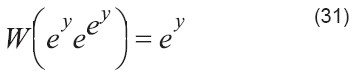
<p ALIGN="justify" style="word-spacing: 0; line-height: 100%"><font size="2" face="Verdana">Identidad:</font></p> </b>     <p ALIGN="justify" style="word-spacing: 0; line-height: 100%"><font size="2" face="Verdana">Igualando las dos soluciones del ejemplo 5 se obtiene:</font></p>     <p ALIGN="center" style="word-spacing: 0; line-height: 100%"><font face="Verdana" size="2"><img border="0" src="/img/fbpe/uct/v10n40/art08ecu38.jpg" width="385" height="45"></font></p>     
<p ALIGN="justify" style="word-spacing: 0; line-height: 100%"><font size="2" face="Verdana">Lo que también se puede expresar en términos de la función de Wrigt:</font></p>     ]]></body>
<body><![CDATA[<p ALIGN="center" style="word-spacing: 0; line-height: 100%"><font face="Verdana" size="2"><img border="0" src="/img/fbpe/uct/v10n40/art08ecu39.jpg" width="373" height="51"></font></p>     
<p ALIGN="justify" style="word-spacing: 0; line-height: 100%"><font size="2" face="Verdana">Por tanto, en general se cumple la identidad:</font></p>     <p ALIGN="center" style="word-spacing: 0; line-height: 100%"><font face="Verdana" size="2"><img border="0" src="/img/fbpe/uct/v10n40/art08ecu40.jpg" width="380" height="36"></font></p> <b>     
<p ALIGN="justify" style="word-spacing: 0; line-height: 100%"><font size="2" face="Verdana">Ejemplo 5</font></p> </b>     <p ALIGN="justify" style="word-spacing: 0; line-height: 100%"><font size="2" face="Verdana">Ecuación:</font></p>     <p ALIGN="center" style="word-spacing: 0; line-height: 100%"><font face="Verdana" size="2"><img border="0" src="/img/fbpe/uct/v10n40/art08ecu41.jpg" width="338" height="66"></font></p>     
<p ALIGN="justify" style="word-spacing: 0; line-height: 100%"><font size="2" face="Verdana">Rescribir la ecuación (41):</font></p>     <p ALIGN="center" style="word-spacing: 0; line-height: 100%"><font face="Verdana" size="2"><img border="0" src="/img/fbpe/uct/v10n40/art08ecu42.jpg" width="354" height="42"></font></p>     
<p ALIGN="justify" style="word-spacing: 0; line-height: 100%"><font size="2" face="Verdana">Aplicar W a ambos lados:</font></p>     <p ALIGN="center" style="word-spacing: 0; line-height: 100%"><font face="Verdana" size="2"><img border="0" src="/img/fbpe/uct/v10n40/art08ecu43.jpg" width="332" height="36"></font></p>     
]]></body>
<body><![CDATA[<p ALIGN="justify" style="word-spacing: 0; line-height: 100%"><font size="2" face="Verdana">Usar definición de W en la parte izquierda:</font></p>     <p ALIGN="center" style="word-spacing: 0; line-height: 100%"><font face="Verdana" size="2"><img border="0" src="/img/fbpe/uct/v10n40/art08ecu44.jpg" width="319" height="53"></font></p>     
<p ALIGN="justify" style="word-spacing: 0; line-height: 100%"><font size="2" face="Verdana">Solución:</font></p>     <p ALIGN="center" style="word-spacing: 0; line-height: 100%"><font face="Verdana" size="2"><img border="0" src="/img/fbpe/uct/v10n40/art08ecu45.jpg" width="325" height="40"></font></p> <b>     
<p ALIGN="justify" style="word-spacing: 0; line-height: 100%"><font size="2" face="Verdana">La función “glog”:</font></p> </b>     <p ALIGN="justify" style="word-spacing: 0; line-height: 100%"><font size="2" face="Verdana">La función glog [35] es la solución a la ecuación (41) que se representa como</font></p>     <p ALIGN="center" style="word-spacing: 0; line-height: 100%"><font face="Verdana" size="2"><img border="0" src="/img/fbpe/uct/v10n40/art08ecu46.jpg" width="331" height="41"></font></p>     
<p ALIGN="justify" style="word-spacing: 0; line-height: 100%"><font size="2" face="Verdana">Comparando las ecuaciones (60) y (61) se puede establecer la equivalencia entre la función de glog y la función de Lambert:</font></p>     <p ALIGN="center" style="word-spacing: 0; line-height: 100%"><font face="Verdana" size="2"><img border="0" src="/img/fbpe/uct/v10n40/art08ecu47.jpg" width="365" height="51"></font></p>     
<p ALIGN="center" style="word-spacing: 0; line-height: 100%"><font face="Verdana" size="2"><img border="0" src="/img/fbpe/uct/v10n40/art08ecu48.jpg" width="364" height="50"></font></p> <b>     
]]></body>
<body><![CDATA[<p ALIGN="justify" style="word-spacing: 0; line-height: 100%"><font size="2" face="Verdana">Ejemplo 6</font></p> </b>     <p ALIGN="justify" style="word-spacing: 0; line-height: 100%"><font size="2" face="Verdana">Ecuación:</font></p>     <p ALIGN="center" style="word-spacing: 0; line-height: 100%"><font face="Verdana" size="2"><img border="0" src="/img/fbpe/uct/v10n40/art08ecu49.jpg" width="302" height="49"></font></p>     
<p ALIGN="justify" style="word-spacing: 0; line-height: 100%"><font size="2" face="Verdana">Tomar la raíz cuadrada:</font></p>     <p ALIGN="center" style="word-spacing: 0; line-height: 100%"><font face="Verdana" size="2"><img border="0" src="/img/fbpe/uct/v10n40/art08ecu50.jpg" width="315" height="53"></font></p>     
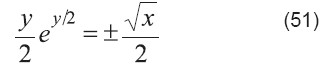
<p ALIGN="justify" style="word-spacing: 0; line-height: 100%"><font size="2" face="Verdana">Dividir entre 2:</font></p>     <p ALIGN="center" style="word-spacing: 0; line-height: 100%"><font face="Verdana" size="2"><img border="0" src="/img/fbpe/uct/v10n40/art08ecu51.jpg" width="325" height="69"></font></p>     
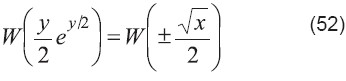
<p ALIGN="justify" style="word-spacing: 0; line-height: 100%"><font size="2" face="Verdana">Aplicar a W a ambos lados:</font></p>     <p ALIGN="center" style="word-spacing: 0; line-height: 100%"><font face="Verdana" size="2"><img border="0" src="/img/fbpe/uct/v10n40/art08ecu52.jpg" width="346" height="81"></font></p>     
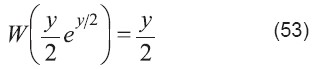
<p ALIGN="justify" style="word-spacing: 0; line-height: 100%"><font size="2" face="Verdana">Usar definición de W en la parte izquierda:</font></p>     ]]></body>
<body><![CDATA[<p ALIGN="center" style="word-spacing: 0; line-height: 100%"><font face="Verdana" size="2"><img border="0" src="/img/fbpe/uct/v10n40/art08ecu53.jpg" width="312" height="69"></font></p>     
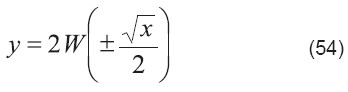
<p ALIGN="justify" style="word-spacing: 0; line-height: 100%"><font size="2" face="Verdana">Solución:</font></p>     <p ALIGN="center" style="word-spacing: 0; line-height: 100%"><font face="Verdana" size="2"><img border="0" src="/img/fbpe/uct/v10n40/art08ecu54.jpg" width="348" height="92"></font></p>     
<p ALIGN="justify" style="word-spacing: 0; line-height: 100%"><font size="2" face="Verdana">Otras ecuaciones tales como x=e<sup>y</sup>/y<sup>2</sup>, x=y<img border="0" src="/img/fbpe/uct/v10n40/art08ecu86.jpg" width="30" height="35">, y=<img border="0" src="/img/fbpe/uct/v10n40/art08ecu87.jpg" width="32" height="32">, etc., pueden resolverse&nbsp;</font>&nbsp;</p>     
<p ALIGN="justify" style="word-spacing: 0; line-height: 100%"><font size="2" face="Verdana">también</font> <font size="2" face="Verdana">usando la función de Lambert.</font></p> <b>     <p ALIGN="justify" style="word-spacing: 0; line-height: 100%"><font size="2" face="Verdana">3. Aplicaciones</font></p> </b>     <p ALIGN="justify" style="word-spacing: 0; line-height: 100%"><font size="2" face="Verdana">Se presentarán ahora varias aplicaciones típicas de la función de Lambert en la solución de diversos problemas de electrónica.</font></p>     <p ALIGN="justify" style="word-spacing: 0; line-height: 100%"><font size="2" face="Verdana">Aunque no se cubrirán todas las posibilidades, se mostrarán algunas que demuestran la solución explícita de circuitos típicos que comúnmente tienen que resolverse mediante aproximaciones o expresiones aproximadas, mientras que otras aplicaciones que se describen pertenecen al ámbito del modelado de dispositivos electrónicos.</font></p> <b>     <p ALIGN="justify" style="word-spacing: 0; line-height: 100%"><font face="Verdana" size="2">3.1 Ruptura irreversible en óxidos de compuerta ultra</font></b><font size="2" face="Verdana"> </font><b><font face="Verdana" size="2">delgados</font></p> </b>     <p ALIGN="justify" style="word-spacing: 0; line-height: 100%"><font size="2" face="Verdana">La continua miniaturización de los dispositivos MOS (Metal Óxido Semiconductor) implica una disminución del margen de confiabilidad de la capacidad aislante de los óxidos de la compuerta que los componen. Ante la posibilidad de que ocurra ruptura eléctrica en óxidos muy delgados, se plantea la necesidad de modelar la corriente que atraviesa el óxido después de su ruptura irreversible. Una representación compacta de esa corriente post ruptura, que es adecuada para la simulación en circuitos, viene dada por el siguiente modelo [19]:</font></p>     ]]></body>
<body><![CDATA[<p ALIGN="center" style="word-spacing: 0; line-height: 100%"><font face="Verdana" size="2"><img border="0" src="/img/fbpe/uct/v10n40/art08ecu55.jpg" width="453" height="42"></font></p>     
<p ALIGN="justify" style="word-spacing: 0; line-height: 100%"><font face="Verdana" size="2">donde I0, <span style="mso-fareast-font-family: Times New Roman; mso-ansi-language: ES; mso-fareast-language: ES; mso-bidi-language: AR-SA">&#969;</span> y RDB son parámetros que caracterizan el fenómeno de ruptura irreversible en una primera aproximación. Esta ecuación equivale a una juntura PN con una resistencia en serie. Rescribiendo la ecuación anterior,</font></p>     <p ALIGN="center" style="word-spacing: 0; line-height: 100%"><font face="Verdana" size="2"><img border="0" src="/img/fbpe/uct/v10n40/art08ecu56.jpg" width="524" height="34"></font></p>     
<p ALIGN="justify" style="word-spacing: 0; line-height: 100%"><font size="2" face="Verdana">Multiplicando ambos lados por y agrupando los términos:</font></p>     <p ALIGN="center" style="word-spacing: 0; line-height: 100%"><font face="Verdana" size="2"><img border="0" src="/img/fbpe/uct/v10n40/art08ecu57.jpg" width="475" height="89"></font></p>     
<p ALIGN="justify" style="word-spacing: 0; line-height: 100%"><font size="2" face="Verdana">Si ahora se aplica W a ambos lados y se usa la definición de W en la parte izquierda de la ecuación, se tiene que</font></p>     <p ALIGN="center" style="word-spacing: 0; line-height: 100%"><font face="Verdana" size="2"><img border="0" src="/img/fbpe/uct/v10n40/art08ecu58.jpg" width="504" height="41"></font></p>     
<p ALIGN="justify" style="word-spacing: 0; line-height: 100%"><font size="2" face="Verdana">Resolviendo resulta la corriente de post ruptura a través del óxido:</font></p>     <p ALIGN="center" style="word-spacing: 0; line-height: 100%"><font face="Verdana" size="2"><img border="0" src="/img/fbpe/uct/v10n40/art08ecu59.jpg" width="497" height="66"></font></p> <b>     
<p ALIGN="justify" style="word-spacing: 0; line-height: 100%"><font size="2" face="Verdana">3.2 Juntura no ideal</font></p> </b>     ]]></body>
<body><![CDATA[<p ALIGN="justify" style="word-spacing: 0; line-height: 100%"><font size="2" face="Verdana">El caso anterior representa el ejemplo más sencillo de una juntura no ideal. Sin embargo, en muchos casos ese modelo resulta ser insuficiente para caracterizar una juntura real. En la <a href="#fig2"><b> Figura 2</b></a> se presenta un modelo circuital genérico de una juntura no ideal, incluyendo sus elementos parásitos más comunes: una conductancia en paralelo que representa la fuga a través de la juntura propiamente dicha (Gp1), una resistencia en serie que da cuenta de la caída de potencial desde la juntura hasta los contactos (Rs), y una segunda conductancia en paralelo que representa la posibilidad de fuga en la periferia del dispositivo (Gp2).</font></p>     <p ALIGN="justify" style="word-spacing: 0; line-height: 100%"><a name="fig2"></a></p>     <p ALIGN="center" style="word-spacing: 0; line-height: 100%"><font face="Verdana" size="2"><img border="0" src="/img/fbpe/uct/v10n40/art08fig2.jpg" width="500" height="355"></font></p> <b>     
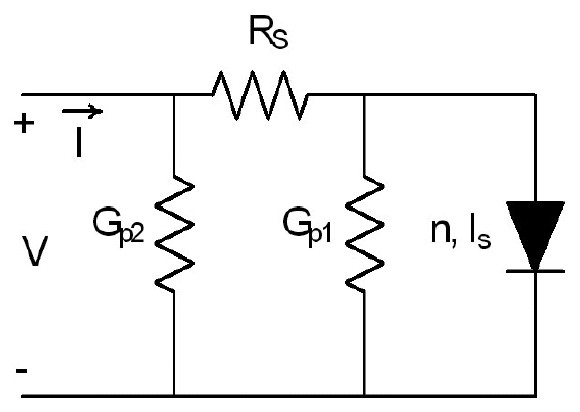
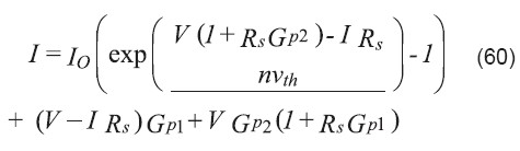
<p ALIGN="center" style="word-spacing: 0; line-height: 100%"><font face="Verdana" size="2">Figura 2. Modelo circuital genérico de una juntura no ideal</font></b><font size="2" face="Verdana"> <b>incluyendo las resistencias en serie y las conductancias en</b>  </font><b><font face="Verdana" size="2">paralelo parásitas.</font></p> </b>     <p ALIGN="justify" style="word-spacing: 0; line-height: 100%"><font size="2" face="Verdana">La ecuación de la corriente que correspondiente a esta configuración es:</font></p>     <p ALIGN="center" style="word-spacing: 0; line-height: 100%"><font face="Verdana" size="2"><img border="0" src="/img/fbpe/uct/v10n40/art08ecu60.jpg" width="475" height="138"></font></p>     
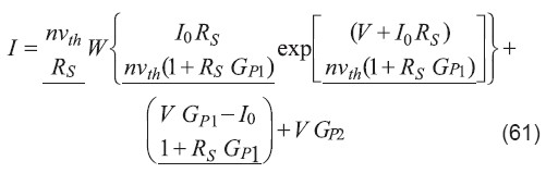
<p ALIGN="justify" style="word-spacing: 0; line-height: 100%"><font size="2" face="Verdana">donde I<sub>0</sub>, es la corriente de saturación inversa del diodo, n es el factor de idealidad que caracteriza la calidad de la juntura, v<sub>th</sub> es el voltaje térmico =kT/q, k la constante de Boltzmann, T la temperatura absoluta, y q la carga electrónica. Nótese que esta ecuación no tiene la forma de una función explícita de una variable en función de la otra y la única manera de resolverla exactamente es mediante iteración numérica. Sin embargo, utilizando la función de Lambert es posible hallar soluciones explícitas de esta ecuación. Siguiendo un procedimiento similar al del ejemplo anterior, la solución de la corriente en función del voltaje resulta ser [13]:</font></p>     <p ALIGN="center" style="word-spacing: 0; line-height: 100%"><font face="Verdana" size="2"><img border="0" src="/img/fbpe/uct/v10n40/art08ecu61.jpg" width="501" height="159"></font></p>     
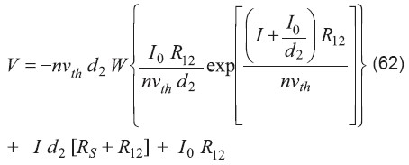
<p ALIGN="justify" style="word-spacing: 0; line-height: 100%"><font size="2" face="Verdana">También es posible resolver el voltaje en función de la corriente:</font></p>     <p ALIGN="center" style="word-spacing: 0; line-height: 100%"><font face="Verdana" size="2"><img border="0" src="/img/fbpe/uct/v10n40/art08ecu62.jpg" width="454" height="183"></font></p>     
]]></body>
<body><![CDATA[<p ALIGN="justify" style="word-spacing: 0; line-height: 100%"><font size="2" face="Verdana">donde:</font></p>     <p ALIGN="center" style="word-spacing: 0; line-height: 100%"><font face="Verdana" size="2"><img border="0" src="/img/fbpe/uct/v10n40/art08ecu63.jpg" width="366" height="56"></font></p>     
<p ALIGN="center" style="word-spacing: 0; line-height: 100%"><font face="Verdana" size="2"><img border="0" src="/img/fbpe/uct/v10n40/art08ecu64.jpg" width="369" height="52"></font></p>     
<p ALIGN="center" style="word-spacing: 0; line-height: 100%"><font face="Verdana" size="2"><img border="0" src="/img/fbpe/uct/v10n40/art08ecu65.jpg" width="444" height="45"></font></p>     
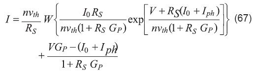
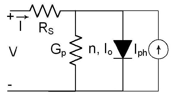
<p ALIGN="justify" style="word-spacing: 0; line-height: 100%"><font size="2" face="Verdana">Estas soluciones explícitas permiten el estudio directo de las características corriente voltaje de junturas no ideales (diodos reales) y facilitan la extracción de los parámetros intrínsecos y extrínsecos de sus modelos [17].</font></p> <b>     <p ALIGN="justify" style="word-spacing: 0; line-height: 100%"><font size="2" face="Verdana">3.3 Celdas solares</font></p> </b>     <p ALIGN="justify" style="word-spacing: 0; line-height: 100%"><font face="Verdana" size="2">Un caso ligeramente más complicado ocurre cuando se intenta modelar celdas solares bajo condiciones de iluminación. En la <a href="#fig3"><b> Figura 3</b></a> se muestra un modelo circuital de un dispositivo fotovoltaico genérico iluminado (celda solar), que incluye la juntura (n, Io), una fuente de corriente fotogenerada (Iph), y la resistencia en serie (Rs) y conductancia en paralelo (Gp) parásitas. La ecuación que describe esta la corriente de la celda es:</font></p>     <p ALIGN="center" style="word-spacing: 0; line-height: 100%"><font face="Verdana" size="2"><img border="0" src="/img/fbpe/uct/v10n40/art08ecu66.jpg" width="503" height="76"></font></p>     
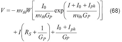
<p ALIGN="justify" style="word-spacing: 0; line-height: 100%"><font size="2" face="Verdana">De nuevo esta ecuación es implícita, pero usando W, se puede hallar la solución explícita para la corriente: y para el voltaje es:</font></p>     <p ALIGN="center" style="word-spacing: 0; line-height: 100%"><font face="Verdana" size="2"><img border="0" src="/img/fbpe/uct/v10n40/art08ecu67.jpg" width="514" height="149"></font></p>     
]]></body>
<body><![CDATA[<p ALIGN="justify" style="word-spacing: 0; line-height: 100%"><font size="2" face="Verdana">y para el voltaje es:</font></p>     <p ALIGN="center" style="word-spacing: 0; line-height: 100%"><font face="Verdana" size="2"><img border="0" src="/img/fbpe/uct/v10n40/art08ecu68.jpg" width="420" height="145"></font></p>     
<p ALIGN="justify" style="word-spacing: 0; line-height: 100%"><font size="2" face="Verdana">La naturaleza explícita de estas soluciones permite calcular inmediatamente la corriente de cortocircuito y el voltaje a circuito abierto. Así mismo, es posible hallar explícitamente el punto de potencia máxima calculando la derivada del producto IV. Estas soluciones también facilitan la extracción de los parámetros del modelo de la celda solar a partir de datos experimentales, como se verá a continuación.</font></p>     <p ALIGN="justify" style="word-spacing: 0; line-height: 100%"><a name="fig3"></a></p>     <p ALIGN="center" style="word-spacing: 0; line-height: 100%"><font face="Verdana" size="2"><img border="0" src="/img/fbpe/uct/v10n40/art08fig3.jpg" width="500" height="275"></font></p> <b>     
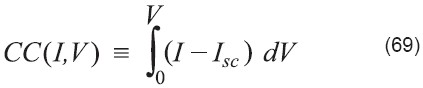
<p ALIGN="center" style="word-spacing: 0; line-height: 100%"><font face="Verdana" size="2">Figura 3. Modelo circuital genérico de una celda solar</font></b><font size="2" face="Verdana"> </font><b><font face="Verdana" size="2">iluminada.</font></p>     <p ALIGN="justify" style="word-spacing: 0; line-height: 100%"><font size="2" face="Verdana">3.4 Extracción de parámetros de modelos de celdas solares</font></p> </b>     <p ALIGN="justify" style="word-spacing: 0; line-height: 100%"><font size="2" face="Verdana">Las técnicas comunes de extracción de parámetros del modelo de la celda solar usando los datos I-V medidos bajo iluminación usualmente incluyen la optimización numérica del error cuadrático en el eje vertical (corriente) o en el eje horizontal (voltaje). La utilización de soluciones explícitas de la corriente y el voltaje facilitan enormemente estos cálculos. Otros métodos están basados en el uso de funciones auxiliares y otros operadores. Aquí se presentará otro método basado en integración, por ser más inmune a los errores de medición debido a su naturaleza de filtro pasa bajo y porque produce resultados algebraicos de fácil manejo computacional [18]. El procedimiento ilustra la utilidad que ofrece la posibilidad de integrar la función de Lambert.</font></p>     <p ALIGN="justify" style="word-spacing: 0; line-height: 100%"><font size="2" face="Verdana">Se define primeramente una función llamada Co-Contenido CC (I,V) de la siguiente manera:</font></p>     <p ALIGN="center" style="word-spacing: 0; line-height: 100%"><font face="Verdana" size="2"><img border="0" src="/img/fbpe/uct/v10n40/art08ecu69.jpg" width="423" height="88"></font></p>     
]]></body>
<body><![CDATA[<p ALIGN="justify" style="word-spacing: 0; line-height: 100%"><font size="2" face="Verdana">donde es la corriente de la celda en condiciones de cortocircuito (V=0). Sustituyendo la solución para la corriente dada por la ecuación (67) en la ecuación de CC e integrando con respecto a V resulta una larga expresión que contiene términos con la función de Lambert y las variables I y V. Reemplazando los términos que contienen la función de Lambert de V, usando la ecuación (68) y después de manipulación y simplificación se obtiene la siguiente ecuación algebraica:</font></p>     <p ALIGN="center" style="word-spacing: 0; line-height: 100%"><font face="Verdana" size="2"><img border="0" src="/img/fbpe/uct/v10n40/art08ecu70.jpg" width="499" height="75"></font></p>     
<p ALIGN="justify" style="word-spacing: 0; line-height: 100%"><font size="2" face="Verdana">donde los cinco coeficientes son funciones de los parámetros del modelo. La extracción se hace calculando la función CC, definida&nbsp; por la ecuación (69), a partir de los datos experimentalmentemedidos. Seguidamente se procede a ajustar esta función de CC a los datos experimentales medidos mediante la ecuación algebraica (70). Este proceso de ajuste bidimensional produce los valores de los coeficientes de la ecuación (70), de los que se calculan los parámetros del modelo G<sub>p</sub>, R<sub>s</sub>, I<sub>ph</sub>, n, y I<sub>o</sub> de la siguiente manera:</font></p>     <p ALIGN="center" style="word-spacing: 0; line-height: 100%"><font face="Verdana" size="2"><img border="0" src="/img/fbpe/uct/v10n40/art08ecu71.jpg" width="382" height="63"></font></p>     
<p ALIGN="center" style="word-spacing: 0; line-height: 100%"><font face="Verdana" size="2"><img border="0" src="/img/fbpe/uct/v10n40/art08ecu72.jpg" width="431" height="80"></font></p>     
<p ALIGN="center" style="word-spacing: 0; line-height: 100%"><font face="Verdana" size="2"><img border="0" src="/img/fbpe/uct/v10n40/art08ecu73.jpg" width="500" height="73"></font></p>     
<p ALIGN="center" style="word-spacing: 0; line-height: 100%"><font face="Verdana" size="2"><img border="0" src="/img/fbpe/uct/v10n40/art08ecu74.jpg" width="504" height="58"></font></p>     
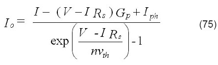
<p ALIGN="center" style="word-spacing: 0; line-height: 100%"><font face="Verdana" size="2"><img border="0" src="/img/fbpe/uct/v10n40/art08ecu75.jpg" width="445" height="134"></font></p> <b>     
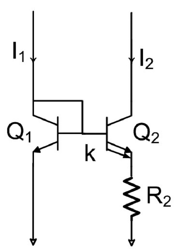
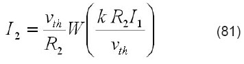
<p ALIGN="justify" style="word-spacing: 0; line-height: 100%"><font size="2" face="Verdana">3.5 Fuente de corriente Widlar</font></p> </b>     <p ALIGN="justify" style="word-spacing: 0; line-height: 100%"><font size="2" face="Verdana">La función de Lambert también es útil en la solución de problemas de circuitos electrónicos con transistores bipolares de juntura. Para ilustrar su utilidad se presentará el caso de la fuente de corriente de Widlar [15] cuyo diagrama circuital básico se muestra en la <b><a href="#fig4"> Figura 4</a></b>.</font></p>     ]]></body>
<body><![CDATA[<p ALIGN="justify" style="word-spacing: 0; line-height: 100%"><font size="2" face="Verdana">En esta fuente de corriente el transistor Q<sub>1</sub> está conectado en configuración de diodo. Se pretende establecer I<sub>2</sub> a partir de los valores de I<sub>1</sub> y R<sub>2</sub>. La ecuación que describe al circuito es:</font></p>     <p ALIGN="center" style="word-spacing: 0; line-height: 100%"><font face="Verdana" size="2"><img border="0" src="/img/fbpe/uct/v10n40/art08ecu76.jpg" width="479" height="95"></font></p>     

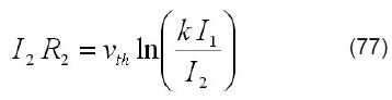
<p ALIGN="center" style="word-spacing: 0; line-height: 100%"><font face="Verdana" size="2"><img border="0" src="/img/fbpe/uct/v10n40/art08ecu77.jpg" width="358" height="92"></font></p>     
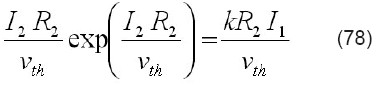
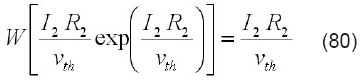
<p ALIGN="justify" style="word-spacing: 0; line-height: 100%"><font size="2" face="Verdana"><span style="mso-fareast-font-family: Times New Roman; mso-bidi-font-family: Times New Roman; mso-ansi-language: ES; mso-fareast-language: ES; mso-bidi-language: AR-SA">Obviamente esta ecuación no expresa a 12 de manera explícita, pues esta corriente aparece también dentro del argumento del logaritmo. La solución habría que hallarla por iteración numérica o usando una aproximación, por ejemplo, los primeros términos de una expansión en serie de Taylor del logaritmo. Se buscará entonces una solución usando la función de Lambert. Tomando exponenciales en ambos lados y multiplicando por 12 R2/vth se obtiene:</span></font></p>     <p ALIGN="center" style="word-spacing: 0; line-height: 100%"><font face="Verdana" size="2"><img border="0" src="/img/fbpe/uct/v10n40/art08ecu78.jpg" width="378" height="86"></font></p>     
<p ALIGN="left" style="word-spacing: 0; line-height: 100%"><a name="fig4"></a></p>     <p ALIGN="center" style="word-spacing: 0; line-height: 100%"><font face="Verdana" size="2"><img border="0" src="/img/fbpe/uct/v10n40/art08fig4.jpg" width="500" height="706"></font></p> <b>     
<p ALIGN="center" style="word-spacing: 0; line-height: 100%"><font size="2" face="Verdana">Figura 4. La fuente de Widlar</font></p> </b>     <p ALIGN="justify" style="word-spacing: 0; line-height: 100%"><font size="2" face="Verdana">Si ahora se aplica la función de Lambert a ambos lados se tiene:</font></p>     <p ALIGN="center" style="word-spacing: 0; line-height: 100%"><font face="Verdana" size="2"><img border="0" src="/img/fbpe/uct/v10n40/art08ecu79.jpg" width="435" height="83"></font></p>     
]]></body>
<body><![CDATA[<p ALIGN="justify" style="word-spacing: 0; line-height: 100%"><font size="2" face="Verdana">pero se sabe que</font></p>     <p ALIGN="center" style="word-spacing: 0; line-height: 100%"><font face="Verdana" size="2"><img border="0" src="/img/fbpe/uct/v10n40/art08ecu80.jpg" width="360" height="82"></font></p>     
<p ALIGN="justify" style="word-spacing: 0; line-height: 100%"><font size="2" face="Verdana">luego, finalmente la corriente I<sub>2</sub> viene dada en forma explícita por</font></p>     <p ALIGN="center" style="word-spacing: 0; line-height: 100%"><font face="Verdana" size="2"><img border="0" src="/img/fbpe/uct/v10n40/art08ecu81.jpg" width="356" height="94"></font></p> <b>     
<p ALIGN="justify" style="word-spacing: 0; line-height: 100%"><font size="2" face="Verdana">3.6 Modelado de dispositivos MOSFET</font></p> </b>     <p ALIGN="justify" style="word-spacing: 0; line-height: 100%"><font size="2" face="Verdana">La descripción del potencial electrostático en la superficie del canal, en función de los voltajes en los terminales de los transistores de efecto de campo tipo metal óxido semiconductor (MOSFETs), resulta de principal importancia en la elaboración de los modelos matemáticos que deben representar a estos dispositivos en simulaciones circuitales. En dispositivos convencionales, en los que el cuerpo del canal se encuentra significativamente dopado, la naturaleza de la ecuación que relaciona el voltaje de la compuerta con el potencial superficial no permite plantear una solución analítica explícita del potencial superficial, por lo que debe calcularse mediante iteración numérica o usando soluciones analíticas aproximadas o de validez limitada regionalmente. Los MOSFETs modernos son cada día más de cuerpo ultra delgado que no se encuentra significativamente dopado, es decir es intrínseco [21]. En esas condiciones la ecuación que relaciona el voltaje de la compuerta con el potencial superficial se reduce a una ecuación lineal exponencial como las anteriormente descritas.</font></p>     <p ALIGN="justify" style="word-spacing: 0; line-height: 100%"><font size="2" face="Verdana">Considérese un dispositivo de cuerpo intrínseco genérico de espesor<b> </b>t<sub>si</sub>. La ecuación para canal n es</font></p>     <p ALIGN="center" style="word-spacing: 0; line-height: 100%"><font face="Verdana" size="2"><img border="0" src="/img/fbpe/uct/v10n40/art08ecu82.jpg" width="482" height="83"></font></p>     
<p ALIGN="center" style="word-spacing: 0; line-height: 100%"><font face="Verdana" size="2"><img border="0" src="/img/fbpe/uct/v10n40/art08ecu83.jpg" width="376" height="96"></font></p>     
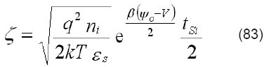
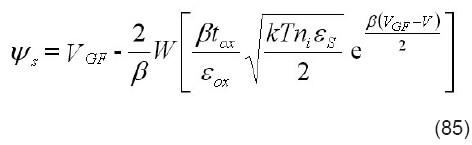
<p ALIGN="justify" style="word-spacing: 0; line-height: 100%"><font size="2" face="Verdana">donde V<sub>G</sub> es el voltaje en la compuerta, V<sub>FB</sub> el voltaje de bandaplana, el potencial superficial, k la constante de Boltzmann, T la temperatura absoluta, ni la densidad intrínseca de portadores, <span style="mso-fareast-font-family: Times New Roman; mso-ansi-language: ES; mso-fareast-language: ES; mso-bidi-language: AR-SA">&#949;</span><sub>s</sub> la permitividad del semiconductor, C<sub>o</sub> la capacitancia del óxido, <span style="mso-fareast-font-family: Times New Roman; mso-ansi-language: ES; mso-fareast-language: ES; mso-bidi-language: AR-SA">&#946;</span>=1/v<sub>th</sub>=q/kT el inverso del voltaje térmico, V el voltaje a lo largo del canal (=0 en el surtidor, =V<sub>D</sub> en el drenador), y <span style="mso-fareast-font-family: Times New Roman; mso-ansi-language: ES; mso-fareast-language: ES; mso-bidi-language: AR-SA">&#968;<sub>0</sub> </span>el potencial en el medio trasversal del canal. Considerando valores de potencial superficial <span style="mso-fareast-font-family: Times New Roman; mso-ansi-language: ES; mso-fareast-language: ES; mso-bidi-language: AR-SA">&#968;<sub>s </sub>&gt;&gt;</span> 1 <span style="mso-fareast-font-family: Times New Roman; mso-ansi-language: ES; mso-fareast-language: ES; mso-bidi-language: AR-SA">&#946;</span>, la ecuación tiene la siguiente solución explícita en base a la función de Lambert:</font></p>     ]]></body>
<body><![CDATA[<p ALIGN="center" style="word-spacing: 0; line-height: 100%"><font face="Verdana" size="2"><img border="0" src="/img/fbpe/uct/v10n40/art08ecu84.jpg" width="497" height="79"></font></p>     
<p ALIGN="justify" style="word-spacing: 0; line-height: 100%"><font face="Verdana" size="2">donde V<sub>GF</sub>=V<sub>G</sub>-V<sub>FB</sub> y t<sub>ox</sub> y <span style="mso-fareast-font-family: Times New Roman; mso-ansi-language: ES; mso-fareast-language: ES; mso-bidi-language: AR-SA">&#949;</span><sub>ox</sub> son el espesor y la permitividad del óxido, respectivamente. Para espesores t<sub>si</sub> del cuerpo del semiconductor muy grandes, <span style="mso-fareast-font-family: Times New Roman; mso-ansi-language: ES; mso-fareast-language: ES; mso-bidi-language: AR-SA">&#968;<sub>0 </sub></span>tiende a cero y el término sin(<span style="mso-fareast-font-family: Times New Roman; mso-ansi-language: ES; mso-fareast-language: ES; mso-bidi-language: AR-SA">&#950;</span>) tiende a uno, con lo que la ecuación del el potencial superficial se reduce a</font></p>     <p ALIGN="center" style="word-spacing: 0; line-height: 100%"><font face="Verdana" size="2"><img border="0" src="/img/fbpe/uct/v10n40/art08ecu85.jpg" width="472" height="145"></font></p>     
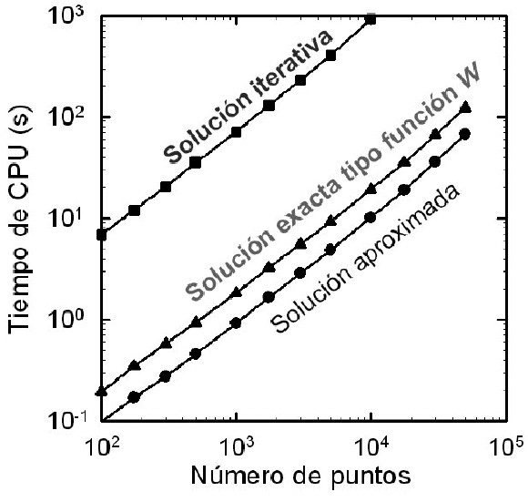
<p ALIGN="justify" style="word-spacing: 0; line-height: 100%"><font size="2" face="Verdana">Esta forma cerrada y explícita de expresar el potencial superficial facilita enormemente el planteamiento de modelos de MOSFETs modernos tipo SOI (semiconductor-óxido-aislante) de cuerpo ultra delgado, en los que el cuerpo del semiconductor no está dopado, tanto los de una compuerta como los de compuertas múltiples [25]. También permite obtener expresiones analíticas explícitas de la carga, la transconductancia, el voltaje de umbral, etc. [23,26].</font></p>     <p ALIGN="justify" style="word-spacing: 0; line-height: 100%"><b><font size="2" face="Verdana">4. Comparación de los tiempos de cómputo</font></b></p>     <p ALIGN="justify" style="word-spacing: 0; line-height: 100%"><font size="2" face="Verdana">Como ya se ha dicho, la utilización de la función de Lambert, además de brindar una alternativa atractiva para la solución explícita exacta de ciertas ecuaciones del tipo lineal exponencial, ofrece la posibilidad de mejorar significativamente la eficiencia computacional, en comparación a las soluciones numéricas iterativas. Para visualizar esta ventaja computacional, es conveniente comparar los tiempos de cálculo requeridos, usando soluciones basadas en la función de Lambert con los de soluciones analíticas aproximadas y soluciones numéricas iterativas. Para esto se usará el caso del modelo de una juntura no ideal con una resistencia en serie y una conductancia en paralelo, calculadas a diez dígitos significativos en una misma plataforma computacional, usando el programa Maple®.</font></p>     <p ALIGN="justify" style="word-spacing: 0; line-height: 100%"><font size="2" face="Verdana">La <b><a href="#fig5"> Figura 5</a></b> muestra que la solución explícita exacta, basada en la función de Lambert, requiere tiempos de CPU sólo ligeramente superiores a los de una solución analítica aproximada, que por ende es inexacta y limitada en su alcance. Se ve que la solución basada en la función de Lambert es casi dos órdenes de magnitud más eficiente computacionalmente que la solución exacta mediante iteración numérica.</font></p>     <p ALIGN="justify" style="word-spacing: 0; line-height: 100%"><a name="fig5"></a></p>     <p ALIGN="center" style="word-spacing: 0; line-height: 100%"><font face="Verdana" size="2"><img border="0" src="/img/fbpe/uct/v10n40/art08fig5.jpg" width="500" height="475"></font></p> <b>     
<p ALIGN="center" style="word-spacing: 0; line-height: 100%"><font face="Verdana" size="2">Figura 5. Comparación de tiempos de cómputo de parámetros</font></b><font size="2" face="Verdana"> <b>del modelo de una juntura no ideal para solución iterativa,</b>  </font><b><font face="Verdana" size="2">exacta y aproximada</font></p>     ]]></body>
<body><![CDATA[<p ALIGN="justify" style="word-spacing: 0; line-height: 100%"><font size="2" face="Verdana">III. CONCLUSIONES</font></p> </b>     <blockquote>       <p ALIGN="justify" style="word-spacing: 0; line-height: 100%"><font size="2" face="Verdana">1.   El uso de la función de Lambert provee soluciones explícitas analíticas y   elimina la necesidad de iteraciones numéricas en problemas que incluyan   ecuaciones implícitas lineales exponenciales.</font></p>       <p ALIGN="justify" style="word-spacing: 0; line-height: 100%"><font size="2" face="Verdana">2.   Las soluciones explícitas basadas en la función de Lambert hacen que el   fenómeno que se está describiendo sea más manejable y fácil de entender.</font></p>       <p ALIGN="justify" style="word-spacing: 0; line-height: 100%"><font size="2" face="Verdana">3.   Estas soluciones explícitas se pueden evaluar y manipular fácilmente, lo que   permite resolver rápidamente numerosos casos repetidos, y facilita el estudio   de las perturbaciones.</font></p>       <p ALIGN="justify" style="word-spacing: 0; line-height: 100%"><font size="2" face="Verdana">4.   La posibilidad de integración y diferenciación analítica de la función de   Lambert abre el camino para elaborar modelos de variabilidad del fenómeno   descrito.</font></p>       <p ALIGN="justify" style="word-spacing: 0; line-height: 100%"><font size="2" face="Verdana">5.   Adicionalmente, estas expresiones explícitas pueden usarse para obtener   suposiciones iniciales para cálculos complicados, iterativos, dependientes   del tiempo, o multi dimensionales.</font></p>       <p ALIGN="justify" style="word-spacing: 0; line-height: 100%"><font size="2" face="Verdana">6.   Finalmente, la utilidad de la función de Lambert se ve potenciada en la   actualidad por la disponibilidad de paquetes computacionales simbólicos de   uso común, tales como Macsyma®, Mathematica®, Maple®, etc., que ya   contienen rutinas optimizadas para calcular y manipular la función de   Lambert.</font></p> </blockquote> <b>     <p ALIGN="justify" style="word-spacing: 0; line-height: 100%"><font size="2" face="Verdana">IV. REFERENCIAS</font></p> </b>     <!-- ref --><p ALIGN="justify" style="word-spacing: 0; line-height: 100%"><font size="2" face="Verdana">1. Corless, R.M., et al., “On the Lambert W Function”. Advances in Computational Mathematics, 5:4, pp. 329–359, 1996.</font>&nbsp;&nbsp;&nbsp;&nbsp;&nbsp;&nbsp;&nbsp;&nbsp;[&#160;<a href="javascript:void(0);" onclick="javascript: window.open('/scielo.php?script=sci_nlinks&ref=2525425&pid=S1316-4821200600040000800001&lng=','','width=640,height=500,resizable=yes,scrollbars=1,menubar=yes,');">Links</a>&#160;]<!-- end-ref --><!-- ref --><p ALIGN="justify" style="word-spacing: 0; line-height: 100%"><font size="2" face="Verdana">2. Gosper, R. W. Jr. &quot;The Solutions of ye<sup>y2</sup>=x and ye<sup>y</sup>=x.&quot; ACM SIGSAM Bull. 32, pp. 8-10, 1998.</font>&nbsp;&nbsp;&nbsp;&nbsp;&nbsp;&nbsp;&nbsp;&nbsp;[&#160;<a href="javascript:void(0);" onclick="javascript: window.open('/scielo.php?script=sci_nlinks&ref=2525426&pid=S1316-4821200600040000800002&lng=','','width=640,height=500,resizable=yes,scrollbars=1,menubar=yes,');">Links</a>&#160;]<!-- end-ref --><!-- ref --><p ALIGN="justify" style="word-spacing: 0; line-height: 100%"><font size="2" face="Verdana">3. Brian Hayes, “Why W?” American Scientist, 93, March-April, p. 104, 2005.</font>&nbsp;&nbsp;&nbsp;&nbsp;&nbsp;&nbsp;&nbsp;&nbsp;[&#160;<a href="javascript:void(0);" onclick="javascript: window.open('/scielo.php?script=sci_nlinks&ref=2525427&pid=S1316-4821200600040000800003&lng=','','width=640,height=500,resizable=yes,scrollbars=1,menubar=yes,');">Links</a>&#160;]<!-- end-ref --><!-- ref --><p ALIGN="justify" style="word-spacing: 0; line-height: 100%"><font size="2" face="Verdana">4. Wright, E. M. &quot;Solution of the Equation ze<sup>z</sup>=<span style="font-size:12.0pt;font-family:&quot;Times New Roman&quot;; mso-fareast-font-family:&quot;Times New Roman&quot;;mso-ansi-language:ES;mso-fareast-language: ES;mso-bidi-language:AR-SA">&#945;</span>.&quot; Bull. Amer. Math. Soc. 65, pp. 89-93, 1959.</font>&nbsp;&nbsp;&nbsp;&nbsp;&nbsp;&nbsp;&nbsp;&nbsp;[&#160;<a href="javascript:void(0);" onclick="javascript: window.open('/scielo.php?script=sci_nlinks&ref=2525428&pid=S1316-4821200600040000800004&lng=','','width=640,height=500,resizable=yes,scrollbars=1,menubar=yes,');">Links</a>&#160;]<!-- end-ref --><!-- ref --><p ALIGN="justify" style="word-spacing: 0; line-height: 100%"><font size="2" face="Verdana">5. Valluri, S. R.; Jeffrey, D. J.; and Corless, R. M. &quot;Some Applications of the Lambert Function to Physics.&quot; Canad. J. Phys. 78, pp. 823-831, 2000.</font>&nbsp;&nbsp;&nbsp;&nbsp;&nbsp;&nbsp;&nbsp;&nbsp;[&#160;<a href="javascript:void(0);" onclick="javascript: window.open('/scielo.php?script=sci_nlinks&ref=2525429&pid=S1316-4821200600040000800005&lng=','','width=640,height=500,resizable=yes,scrollbars=1,menubar=yes,');">Links</a>&#160;]<!-- end-ref --><!-- ref --><p ALIGN="justify" style="word-spacing: 0; line-height: 100%"><font size="2" face="Verdana">6. Jenn, D.C., “Applications of the Lambert W Function in Electromagnetics” IEEE Antennas and Propagation Magazine, 44, pp. 139-142, 2002.</font>&nbsp;&nbsp;&nbsp;&nbsp;&nbsp;&nbsp;&nbsp;&nbsp;[&#160;<a href="javascript:void(0);" onclick="javascript: window.open('/scielo.php?script=sci_nlinks&ref=2525430&pid=S1316-4821200600040000800006&lng=','','width=640,height=500,resizable=yes,scrollbars=1,menubar=yes,');">Links</a>&#160;]<!-- end-ref --><!-- ref --><p ALIGN="justify" style="word-spacing: 0; line-height: 100%"><font size="2" face="Verdana">7. Jean-Michel Caillol, “Some Applications of the Lambert W Function to Classical Statistical Mechanics”, J. Phys. A: Math. Gen. 36, pp. 10431-10442, 2003.</font>&nbsp;&nbsp;&nbsp;&nbsp;&nbsp;&nbsp;&nbsp;&nbsp;[&#160;<a href="javascript:void(0);" onclick="javascript: window.open('/scielo.php?script=sci_nlinks&ref=2525431&pid=S1316-4821200600040000800007&lng=','','width=640,height=500,resizable=yes,scrollbars=1,menubar=yes,');">Links</a>&#160;]<!-- end-ref --><!-- ref --><p ALIGN="justify" style="word-spacing: 0; line-height: 100%"><font size="2" face="Verdana">8. Packel, E. and Yuen, D. &quot;Projectile Motion with Resistance and the Lambert Function.&quot; College Math. J., 35, pp. 337- 350, 2004.</font>&nbsp;&nbsp;&nbsp;&nbsp;&nbsp;&nbsp;&nbsp;&nbsp;[&#160;<a href="javascript:void(0);" onclick="javascript: window.open('/scielo.php?script=sci_nlinks&ref=2525432&pid=S1316-4821200600040000800008&lng=','','width=640,height=500,resizable=yes,scrollbars=1,menubar=yes,');">Links</a>&#160;]<!-- end-ref --><!-- ref --><p ALIGN="justify" style="word-spacing: 0; line-height: 100%"><font size="2" face="Verdana">9. Chapeau-Blondeau, F. Monir, A. “Numerical Evaluation of the Lambert W Function and Application to Generation of Generalized Gaussian Noise With Exponent ½”, IEEE Trans. Signal Proc., 50; Part 9, pp. 2160-2165, 2002.</font>&nbsp;&nbsp;&nbsp;&nbsp;&nbsp;&nbsp;&nbsp;&nbsp;[&#160;<a href="javascript:void(0);" onclick="javascript: window.open('/scielo.php?script=sci_nlinks&ref=2525433&pid=S1316-4821200600040000800009&lng=','','width=640,height=500,resizable=yes,scrollbars=1,menubar=yes,');">Links</a>&#160;]<!-- end-ref --><!-- ref --><p ALIGN="justify" style="word-spacing: 0; line-height: 100%"><font size="2" face="Verdana">10. Barry, D. A., Li, L., Jeng, D.S. , “Comments on ‘Numerical Evaluation of the Lambert Function and Application to Generation of Generalized Gaussian Noise with Exponent ½’” IEEE Trans. on Signal Processing, 52, pp. 1456-1458, 2004.</font>&nbsp;&nbsp;&nbsp;&nbsp;&nbsp;&nbsp;&nbsp;&nbsp;[&#160;<a href="javascript:void(0);" onclick="javascript: window.open('/scielo.php?script=sci_nlinks&ref=2525434&pid=S1316-4821200600040000800010&lng=','','width=640,height=500,resizable=yes,scrollbars=1,menubar=yes,');">Links</a>&#160;]<!-- end-ref --><!-- ref --><p ALIGN="justify" style="word-spacing: 0; line-height: 100%"><font size="2" face="Verdana">11. I.N. Galidakis, “On an Application of Lambert's W Function to Infinite Exponentials”, Complex Variables, 49(11), pp. 759- 780, 2004.</font>&nbsp;&nbsp;&nbsp;&nbsp;&nbsp;&nbsp;&nbsp;&nbsp;[&#160;<a href="javascript:void(0);" onclick="javascript: window.open('/scielo.php?script=sci_nlinks&ref=2525435&pid=S1316-4821200600040000800011&lng=','','width=640,height=500,resizable=yes,scrollbars=1,menubar=yes,');">Links</a>&#160;]<!-- end-ref --><!-- ref --><p ALIGN="justify" style="word-spacing: 0; line-height: 100%"><font size="2" face="Verdana">12. Brian Wesley Williams, “Exact Solutions of a Schrödinger Equation Based on the Lambert Function”, Physics Letters A, 334(2-3), pp. 117-122, 2005.</font>&nbsp;&nbsp;&nbsp;&nbsp;&nbsp;&nbsp;&nbsp;&nbsp;[&#160;<a href="javascript:void(0);" onclick="javascript: window.open('/scielo.php?script=sci_nlinks&ref=2525436&pid=S1316-4821200600040000800012&lng=','','width=640,height=500,resizable=yes,scrollbars=1,menubar=yes,');">Links</a>&#160;]<!-- end-ref --><!-- ref --><p ALIGN="justify" style="word-spacing: 0; line-height: 100%"><font size="2" face="Verdana">13. Ortiz-Conde, A., García Sánchez, F.J., Muci, J., “Exact Analytical Solutions of the Forward Non-Ideal Diode Equation with Series and Shunt Parasitic Resistances” Solid-State Electronics, 44, pp. 1861-1864, 2000.</font>&nbsp;&nbsp;&nbsp;&nbsp;&nbsp;&nbsp;&nbsp;&nbsp;[&#160;<a href="javascript:void(0);" onclick="javascript: window.open('/scielo.php?script=sci_nlinks&ref=2525437&pid=S1316-4821200600040000800013&lng=','','width=640,height=500,resizable=yes,scrollbars=1,menubar=yes,');">Links</a>&#160;]<!-- end-ref --><!-- ref --><p ALIGN="justify" style="word-spacing: 0; line-height: 100%"><font size="2" face="Verdana">14. Banwell, T. C. and Jayakumar, A. &quot;Exact Analytical Solution for Current Flow Through Diode with Series Resistance.&quot; Electronics Lett. 36, pp. 291-292, 2000.</font>&nbsp;&nbsp;&nbsp;&nbsp;&nbsp;&nbsp;&nbsp;&nbsp;[&#160;<a href="javascript:void(0);" onclick="javascript: window.open('/scielo.php?script=sci_nlinks&ref=2525438&pid=S1316-4821200600040000800014&lng=','','width=640,height=500,resizable=yes,scrollbars=1,menubar=yes,');">Links</a>&#160;]<!-- end-ref --><!-- ref --><p ALIGN="justify" style="word-spacing: 0; line-height: 100%"><font size="2" face="Verdana">15. Banwell, T.C., “Bipolar Transistor Circuit Analysis Using the Lambert W-Function” IEEE Trans. Circuits System - I: Fundamental Theory and Applications, 47, pp. 1621-1633, 2000.</font>&nbsp;&nbsp;&nbsp;&nbsp;&nbsp;&nbsp;&nbsp;&nbsp;[&#160;<a href="javascript:void(0);" onclick="javascript: window.open('/scielo.php?script=sci_nlinks&ref=2525439&pid=S1316-4821200600040000800015&lng=','','width=640,height=500,resizable=yes,scrollbars=1,menubar=yes,');">Links</a>&#160;]<!-- end-ref --><!-- ref --><p ALIGN="justify" style="word-spacing: 0; line-height: 100%"><font size="2" face="Verdana">16. A. Jain and A. Kapoor, “Exact Analytical Solutions of the Parameters of Real Solar Cells Using Lambert W Function” Solar Energy Materials and Solar Cells, 81, pp. 269-277, 2004.</font>&nbsp;&nbsp;&nbsp;&nbsp;&nbsp;&nbsp;&nbsp;&nbsp;[&#160;<a href="javascript:void(0);" onclick="javascript: window.open('/scielo.php?script=sci_nlinks&ref=2525440&pid=S1316-4821200600040000800016&lng=','','width=640,height=500,resizable=yes,scrollbars=1,menubar=yes,');">Links</a>&#160;]<!-- end-ref --><!-- ref --><p ALIGN="justify" style="word-spacing: 0; line-height: 100%"><font size="2" face="Verdana">17. Ortiz-Conde, A., García Sánchez, F.J., “Extraction of Non- Ideal Junction Model Parameters from the Explicit Analytic Solutions of its I–V Characteristics” Solid-State Electronics 49, pp. 465–472, 2005.</font>&nbsp;&nbsp;&nbsp;&nbsp;&nbsp;&nbsp;&nbsp;&nbsp;[&#160;<a href="javascript:void(0);" onclick="javascript: window.open('/scielo.php?script=sci_nlinks&ref=2525441&pid=S1316-4821200600040000800017&lng=','','width=640,height=500,resizable=yes,scrollbars=1,menubar=yes,');">Links</a>&#160;]<!-- end-ref --><!-- ref --><p ALIGN="justify" style="word-spacing: 0; line-height: 100%"><font size="2" face="Verdana">18. [18] Ortiz-Conde, A., García Sánchez, F.J., Muci, J., “New Method to Extract the Model Parameters of Solar Cells from the Explicit Analytic Solutions of their Illuminated I–V Characteristics” Solar Energy Materials &amp; Solar Cells, 90, pp. 352–361, 2006.</font>&nbsp;&nbsp;&nbsp;&nbsp;&nbsp;&nbsp;&nbsp;&nbsp;[&#160;<a href="javascript:void(0);" onclick="javascript: window.open('/scielo.php?script=sci_nlinks&ref=2525442&pid=S1316-4821200600040000800018&lng=','','width=640,height=500,resizable=yes,scrollbars=1,menubar=yes,');">Links</a>&#160;]<!-- end-ref --><!-- ref --><p ALIGN="justify" style="word-spacing: 0; line-height: 100%"><font size="2" face="Verdana">19. Miranda, E., Ortiz-Conde, A., García Sánchez, F.J., Farkas, E., “Extraction of Parameters and Simulation of the Hard Breakdown I-V Characteristics in Ultrathin Gate Oxides” Proceedings of 12th IPFA 2005, Singapore, pp. 150-154, 2005.</font>&nbsp;&nbsp;&nbsp;&nbsp;&nbsp;&nbsp;&nbsp;&nbsp;[&#160;<a href="javascript:void(0);" onclick="javascript: window.open('/scielo.php?script=sci_nlinks&ref=2525443&pid=S1316-4821200600040000800019&lng=','','width=640,height=500,resizable=yes,scrollbars=1,menubar=yes,');">Links</a>&#160;]<!-- end-ref --><!-- ref --><p ALIGN="justify" style="word-spacing: 0; line-height: 100%"><font size="2" face="Verdana">20. Benton H. Calhoun, Alice Wang, and Anantha Chandrakasan, “Modeling and Sizing for Minimum Energy Operation in Subthreshold Circuits” IEEE Journal of Solid-State Circuits, 40, pp. 1778-1886, 2005.</font>&nbsp;&nbsp;&nbsp;&nbsp;&nbsp;&nbsp;&nbsp;&nbsp;[&#160;<a href="javascript:void(0);" onclick="javascript: window.open('/scielo.php?script=sci_nlinks&ref=2525444&pid=S1316-4821200600040000800020&lng=','','width=640,height=500,resizable=yes,scrollbars=1,menubar=yes,');">Links</a>&#160;]<!-- end-ref --><!-- ref --><p ALIGN="justify" style="word-spacing: 0; line-height: 100%"><font size="2" face="Verdana">21. Ortiz-Conde, A., García Sánchez, F.J., &quot;Exact Analytical Solution of Channel Surface Potential as an Explicit Function of Gate Voltage in Undoped-Body Mosfets Using The Lambert W Function and a Threshold Voltage Definition Therefrom“, Solid-State Electronics, 47, Pp. 2067-2074, 2003.</font>&nbsp;&nbsp;&nbsp;&nbsp;&nbsp;&nbsp;&nbsp;&nbsp;[&#160;<a href="javascript:void(0);" onclick="javascript: window.open('/scielo.php?script=sci_nlinks&ref=2525445&pid=S1316-4821200600040000800021&lng=','','width=640,height=500,resizable=yes,scrollbars=1,menubar=yes,');">Links</a>&#160;]<!-- end-ref --><!-- ref --><p ALIGN="justify" style="word-spacing: 0; line-height: 100%"><font size="2" face="Verdana">22. He J., et al., ”Charge-Based Core and the Model Architecture of BSIM5” Proceedings of the Sixth International Symposium on Quality of Electronic Design (ISQED'05), pp. 96-101, 2005.</font>&nbsp;&nbsp;&nbsp;&nbsp;&nbsp;&nbsp;&nbsp;&nbsp;[&#160;<a href="javascript:void(0);" onclick="javascript: window.open('/scielo.php?script=sci_nlinks&ref=2525446&pid=S1316-4821200600040000800022&lng=','','width=640,height=500,resizable=yes,scrollbars=1,menubar=yes,');">Links</a>&#160;]<!-- end-ref --><!-- ref --><p ALIGN="justify" style="word-spacing: 0; line-height: 100%"><font size="2" face="Verdana">23. García-Sánchez, F.J., Ortiz-Conde, A., Muci J., “Subthreshold Behavior of Undoped DG MOSFETs,” Proc of the 2005 IEEE International Conference on Electron Devices and Solid-State Circuits (EDSSC 2005), Hong Kong, pp. 75-80, December 2005.</font>&nbsp;&nbsp;&nbsp;&nbsp;&nbsp;&nbsp;&nbsp;&nbsp;[&#160;<a href="javascript:void(0);" onclick="javascript: window.open('/scielo.php?script=sci_nlinks&ref=2525447&pid=S1316-4821200600040000800023&lng=','','width=640,height=500,resizable=yes,scrollbars=1,menubar=yes,');">Links</a>&#160;]<!-- end-ref --><!-- ref --><p ALIGN="justify" style="word-spacing: 0; line-height: 100%"><font size="2" face="Verdana">24. Giorgio Mugnaini and Giuseppe Iannaccone, “Physics-Based Compact Model of Nanoscale MOSFETs-Part I: Transition From Drift-Diffusion to Ballistic Transport” IEEE Trans. Electron Devices, 52, pp. 1795-1801, 2005.</font>&nbsp;&nbsp;&nbsp;&nbsp;&nbsp;&nbsp;&nbsp;&nbsp;[&#160;<a href="javascript:void(0);" onclick="javascript: window.open('/scielo.php?script=sci_nlinks&ref=2525448&pid=S1316-4821200600040000800024&lng=','','width=640,height=500,resizable=yes,scrollbars=1,menubar=yes,');">Links</a>&#160;]<!-- end-ref --><!-- ref --><p ALIGN="justify" style="word-spacing: 0; line-height: 100%"><font size="2" face="Verdana">25. Ortiz-Conde, A., García Sánchez, F.J. , and Malobabic, S., “Analytic Solution of the Channel Potential in Undoped Symmetric Dual-Gate MOSFETs”, IEEE Trans. Electron Devices, 52, pp. 1669-1672, 2005.</font>&nbsp;&nbsp;&nbsp;&nbsp;&nbsp;&nbsp;&nbsp;&nbsp;[&#160;<a href="javascript:void(0);" onclick="javascript: window.open('/scielo.php?script=sci_nlinks&ref=2525449&pid=S1316-4821200600040000800025&lng=','','width=640,height=500,resizable=yes,scrollbars=1,menubar=yes,');">Links</a>&#160;]<!-- end-ref --><!-- ref --><p ALIGN="justify" style="word-spacing: 0; line-height: 100%"><font size="2" face="Verdana">26. García Sánchez, F.J., Ortiz-Conde, A., Muci, J., “Understanding Threshold Voltage in Undoped-Body Mosfets: An Appraisal of Various Criteria” Microelectronics Reliability, 46, pp. 731-742, 2006.</font>&nbsp;&nbsp;&nbsp;&nbsp;&nbsp;&nbsp;&nbsp;&nbsp;[&#160;<a href="javascript:void(0);" onclick="javascript: window.open('/scielo.php?script=sci_nlinks&ref=2525450&pid=S1316-4821200600040000800026&lng=','','width=640,height=500,resizable=yes,scrollbars=1,menubar=yes,');">Links</a>&#160;]<!-- end-ref --><!-- ref --><p ALIGN="justify" style="word-spacing: 0; line-height: 100%"><font size="2" face="Verdana">27. Jeffrey, D. J.; Hare, D. E. G.; and Corless, R. M. &quot;Unwinding the Branches of the Lambert W Function.&quot; Math. Scientist, 21, pp. 1-7, 1996.</font>&nbsp;&nbsp;&nbsp;&nbsp;&nbsp;&nbsp;&nbsp;&nbsp;[&#160;<a href="javascript:void(0);" onclick="javascript: window.open('/scielo.php?script=sci_nlinks&ref=2525451&pid=S1316-4821200600040000800027&lng=','','width=640,height=500,resizable=yes,scrollbars=1,menubar=yes,');">Links</a>&#160;]<!-- end-ref --><!-- ref --><p ALIGN="justify" style="word-spacing: 0; line-height: 100%"><font size="2" face="Verdana">28. Corless, R. M.; Jeffrey, D. J.; and Knuth, D. E. &quot;A Sequence of Series for the Lambert W Function.&quot; Proc. of the 1997 Intnl Symp. on Symbolic and Algebraic Computation, Maui, Hawaii. New York: ACM Press, pp. 197-204, 1997.</font>&nbsp;&nbsp;&nbsp;&nbsp;&nbsp;&nbsp;&nbsp;&nbsp;[&#160;<a href="javascript:void(0);" onclick="javascript: window.open('/scielo.php?script=sci_nlinks&ref=2525452&pid=S1316-4821200600040000800028&lng=','','width=640,height=500,resizable=yes,scrollbars=1,menubar=yes,');">Links</a>&#160;]<!-- end-ref --><!-- ref --><p ALIGN="justify" style="word-spacing: 0; line-height: 100%"><font size="2" face="Verdana">29. Fritsch, F. N.; Shafer, R. E.; and Crowley, W. P. &quot;Algorithm 443: Solution of the Transcendental Equation we<sup>w</sup>=x.&quot; Comm. ACM ,16, pp. 123-124, 1973.</font>&nbsp;&nbsp;&nbsp;&nbsp;&nbsp;&nbsp;&nbsp;&nbsp;[&#160;<a href="javascript:void(0);" onclick="javascript: window.open('/scielo.php?script=sci_nlinks&ref=2525453&pid=S1316-4821200600040000800029&lng=','','width=640,height=500,resizable=yes,scrollbars=1,menubar=yes,');">Links</a>&#160;]<!-- end-ref --><!-- ref --><p ALIGN="justify" style="word-spacing: 0; line-height: 100%"><font size="2" face="Verdana">30. Barry, D. A., Barry, S. J., Culligan-Hensley, P. J., “Algorithm 743: WAPR: a FORTRAN Routine for Calculating Real Values of the W-Function,” ACM Trans. Math. Softw., 21, pp. 172–181, 1995.</font>&nbsp;&nbsp;&nbsp;&nbsp;&nbsp;&nbsp;&nbsp;&nbsp;[&#160;<a href="javascript:void(0);" onclick="javascript: window.open('/scielo.php?script=sci_nlinks&ref=2525454&pid=S1316-4821200600040000800030&lng=','','width=640,height=500,resizable=yes,scrollbars=1,menubar=yes,');">Links</a>&#160;]<!-- end-ref --><!-- ref --><p ALIGN="justify" style="word-spacing: 0; line-height: 100%"><font size="2" face="Verdana">31. Barry, D. J., Culligen-Hensley, P. J.; and Barry S. J. &quot;Real Values of the W-Function,” ACM Trans. Math. Softw., 21, pp. 161-171, 1995.</font>&nbsp;&nbsp;&nbsp;&nbsp;&nbsp;&nbsp;&nbsp;&nbsp;[&#160;<a href="javascript:void(0);" onclick="javascript: window.open('/scielo.php?script=sci_nlinks&ref=2525455&pid=S1316-4821200600040000800031&lng=','','width=640,height=500,resizable=yes,scrollbars=1,menubar=yes,');">Links</a>&#160;]<!-- end-ref --><!-- ref --><p ALIGN="justify" style="word-spacing: 0; line-height: 100%"><font size="2" face="Verdana">32. D.A. Barry., et al., &quot;Analytical Approximations for Real Values of the Lambert W-function&quot; Mathematics and Computers in Simulation, 53, pp. 95-103, 2000.</font>&nbsp;&nbsp;&nbsp;&nbsp;&nbsp;&nbsp;&nbsp;&nbsp;[&#160;<a href="javascript:void(0);" onclick="javascript: window.open('/scielo.php?script=sci_nlinks&ref=2525456&pid=S1316-4821200600040000800032&lng=','','width=640,height=500,resizable=yes,scrollbars=1,menubar=yes,');">Links</a>&#160;]<!-- end-ref --><!-- ref --><p ALIGN="justify" style="word-spacing: 0; line-height: 100%"><font size="2" face="Verdana">33. J.P. Body, &quot;Global Approximations to the Principal Real-Valued Branch of The Lambert W- Function,&quot; Appl. Math. Lett. 11 (6). Pp. 27-31, 1998.</font>&nbsp;&nbsp;&nbsp;&nbsp;&nbsp;&nbsp;&nbsp;&nbsp;[&#160;<a href="javascript:void(0);" onclick="javascript: window.open('/scielo.php?script=sci_nlinks&ref=2525457&pid=S1316-4821200600040000800033&lng=','','width=640,height=500,resizable=yes,scrollbars=1,menubar=yes,');">Links</a>&#160;]<!-- end-ref --><!-- ref --><p ALIGN="justify" style="word-spacing: 0; line-height: 100%"><font size="2" face="Verdana">34. Corless, R. M. and Jeffrey, D. J. &quot;The Wright <span style="font-size:12.0pt;font-family:&quot;Times New Roman&quot;; mso-fareast-font-family:&quot;Times New Roman&quot;;mso-ansi-language:ES;mso-fareast-language: ES;mso-bidi-language:AR-SA">&#969; </span><span style="mso-fareast-font-family: Times New Roman; mso-ansi-language: ES; mso-fareast-language: ES; mso-bidi-language: AR-SA">Function.&quot; Artificial Intelligence, Automated Reasoning, and Symbolic Computation (Ed. J. Calmet, B. Benhamou, O. Caprotti, L. Henocque and V. Sorge). Berlin: Springer-Verlag, pp. 76-89, 2002.</span></font>&nbsp;&nbsp;&nbsp;&nbsp;&nbsp;&nbsp;&nbsp;&nbsp;[&#160;<a href="javascript:void(0);" onclick="javascript: window.open('/scielo.php?script=sci_nlinks&ref=2525458&pid=S1316-4821200600040000800034&lng=','','width=640,height=500,resizable=yes,scrollbars=1,menubar=yes,');">Links</a>&#160;]<!-- end-ref --><!-- ref --><p ALIGN="justify" style="word-spacing: 0; line-height: 100%"><font size="2" face="Verdana"><span style="mso-fareast-font-family: Times New Roman; mso-ansi-language: ES; mso-fareast-language: ES; mso-bidi-language: AR-SA">35. Kalman, D. &quot;A Generalized Logarithm for Exponential-Linear Equations.&quot; College Math. J., 32, pp. 2-14, 2001.</span></font>&nbsp;&nbsp;&nbsp;&nbsp;&nbsp;&nbsp;&nbsp;&nbsp;[&#160;<a href="javascript:void(0);" onclick="javascript: window.open('/scielo.php?script=sci_nlinks&ref=2525459&pid=S1316-4821200600040000800035&lng=','','width=640,height=500,resizable=yes,scrollbars=1,menubar=yes,');">Links</a>&#160;]<!-- end-ref --> ]]></body>
<back>
<ref-list>
<ref id="B1">
<label>1</label><nlm-citation citation-type="journal">
<person-group person-group-type="author">
<name>
<surname><![CDATA[Corless]]></surname>
<given-names><![CDATA[R.M]]></given-names>
</name>
</person-group>
<article-title xml:lang="en"><![CDATA[On the Lambert W Function]]></article-title>
<source><![CDATA[Advances in Computational Mathematics]]></source>
<year>1996</year>
<volume>5</volume>
<numero>4</numero>
<issue>4</issue>
<page-range>329-359</page-range></nlm-citation>
</ref>
<ref id="B2">
<label>2</label><nlm-citation citation-type="journal">
<person-group person-group-type="author">
<name>
<surname><![CDATA[Gosper]]></surname>
<given-names><![CDATA[R. W. Jr]]></given-names>
</name>
</person-group>
<article-title xml:lang="en"><![CDATA[The Solutions of ye y2=x and ye y=x]]></article-title>
<source><![CDATA[ACM SIGSAM Bull]]></source>
<year>1998</year>
<volume>32</volume>
<page-range>8-10</page-range></nlm-citation>
</ref>
<ref id="B3">
<label>3</label><nlm-citation citation-type="journal">
<person-group person-group-type="author">
<name>
<surname><![CDATA[Hayes]]></surname>
<given-names><![CDATA[Brian]]></given-names>
</name>
</person-group>
<article-title xml:lang="en"><![CDATA[Why W?]]></article-title>
<source><![CDATA[American Scientist]]></source>
<year>2005</year>
<volume>93</volume>
<page-range>104</page-range></nlm-citation>
</ref>
<ref id="B4">
<label>4</label><nlm-citation citation-type="journal">
<person-group person-group-type="author">
<name>
<surname><![CDATA[Wright]]></surname>
<given-names><![CDATA[E. M]]></given-names>
</name>
</person-group>
<article-title xml:lang="en"><![CDATA[Solution of the Equation ze z=&#945;]]></article-title>
<source><![CDATA[Bull. Amer. Math. Soc]]></source>
<year>1959</year>
<volume>65</volume>
<page-range>89-93</page-range></nlm-citation>
</ref>
<ref id="B5">
<label>5</label><nlm-citation citation-type="journal">
<person-group person-group-type="author">
<name>
<surname><![CDATA[Valluri]]></surname>
<given-names><![CDATA[S. R]]></given-names>
</name>
<name>
<surname><![CDATA[Jeffrey]]></surname>
<given-names><![CDATA[D. J]]></given-names>
</name>
<name>
<surname><![CDATA[Corless]]></surname>
<given-names><![CDATA[R. M]]></given-names>
</name>
</person-group>
<article-title xml:lang="en"><![CDATA[Some Applications of the Lambert Function to Physics]]></article-title>
<source><![CDATA[Canad. J. Phys]]></source>
<year>2000</year>
<volume>78</volume>
<page-range>823-831</page-range></nlm-citation>
</ref>
<ref id="B6">
<label>6</label><nlm-citation citation-type="journal">
<person-group person-group-type="author">
<name>
<surname><![CDATA[Jenn]]></surname>
<given-names><![CDATA[D.C]]></given-names>
</name>
</person-group>
<article-title xml:lang="en"><![CDATA[Applications of the Lambert W Function in Electromagnetics]]></article-title>
<source><![CDATA[IEEE Antennas and Propagation Magazine]]></source>
<year>2002</year>
<volume>44</volume>
<page-range>139-142</page-range></nlm-citation>
</ref>
<ref id="B7">
<label>7</label><nlm-citation citation-type="journal">
<person-group person-group-type="author">
<name>
<surname><![CDATA[Caillol]]></surname>
<given-names><![CDATA[Jean-Michel]]></given-names>
</name>
</person-group>
<article-title xml:lang="en"><![CDATA[Some Applications of the Lambert W Function to Classical Statistical Mechanics]]></article-title>
<source><![CDATA[J. Phys. A: Math. Gen]]></source>
<year>2003</year>
<volume>36</volume>
<page-range>10431-10442</page-range></nlm-citation>
</ref>
<ref id="B8">
<label>8</label><nlm-citation citation-type="journal">
<person-group person-group-type="author">
<name>
<surname><![CDATA[Packel]]></surname>
<given-names><![CDATA[E]]></given-names>
</name>
<name>
<surname><![CDATA[Yuen]]></surname>
<given-names><![CDATA[D]]></given-names>
</name>
</person-group>
<article-title xml:lang="en"><![CDATA[Projectile Motion with Resistance and the Lambert Function]]></article-title>
<source><![CDATA[College Math. J]]></source>
<year>2004</year>
<volume>35</volume>
<page-range>337- 350</page-range></nlm-citation>
</ref>
<ref id="B9">
<label>9</label><nlm-citation citation-type="journal">
<person-group person-group-type="author">
<name>
<surname><![CDATA[Chapeau-Blondeau]]></surname>
<given-names><![CDATA[F]]></given-names>
</name>
<name>
<surname><![CDATA[Monir]]></surname>
<given-names><![CDATA[A]]></given-names>
</name>
</person-group>
<article-title xml:lang="en"><![CDATA[Numerical Evaluation of the Lambert W Function and Application to Generation of Generalized Gaussian Noise With Exponent ½]]></article-title>
<source><![CDATA[IEEE Trans. Signal Proc]]></source>
<year>2002</year>
<volume>50</volume>
<page-range>2160-2165</page-range></nlm-citation>
</ref>
<ref id="B10">
<label>10</label><nlm-citation citation-type="journal">
<person-group person-group-type="author">
<name>
<surname><![CDATA[Barry]]></surname>
<given-names><![CDATA[D. A]]></given-names>
</name>
<name>
<surname><![CDATA[Li]]></surname>
<given-names><![CDATA[L]]></given-names>
</name>
<name>
<surname><![CDATA[Jeng]]></surname>
<given-names><![CDATA[D.S]]></given-names>
</name>
</person-group>
<article-title xml:lang="en"><![CDATA[Comments on ‘Numerical Evaluation of the Lambert Function and Application to Generation of Generalized Gaussian Noise with Exponent ½’]]></article-title>
<source><![CDATA[IEEE Trans. on Signal Processing]]></source>
<year>2004</year>
<volume>52</volume>
<page-range>1456-1458</page-range></nlm-citation>
</ref>
<ref id="B11">
<label>11</label><nlm-citation citation-type="journal">
<person-group person-group-type="author">
<name>
<surname><![CDATA[Galidakis]]></surname>
<given-names><![CDATA[I.N]]></given-names>
</name>
</person-group>
<article-title xml:lang="en"><![CDATA[On an Application of Lambert's W Function to Infinite Exponentials]]></article-title>
<source><![CDATA[Complex Variables]]></source>
<year>2004</year>
<volume>49</volume>
<numero>11</numero>
<issue>11</issue>
<page-range>759- 780</page-range></nlm-citation>
</ref>
<ref id="B12">
<label>12</label><nlm-citation citation-type="journal">
<person-group person-group-type="author">
<name>
<surname><![CDATA[Wesley Williams]]></surname>
<given-names><![CDATA[Brian]]></given-names>
</name>
</person-group>
<article-title xml:lang="en"><![CDATA[Exact Solutions of a Schrödinger Equation Based on the Lambert Function]]></article-title>
<source><![CDATA[Physics Letters A]]></source>
<year>2005</year>
<volume>334</volume>
<numero>2-3</numero>
<issue>2-3</issue>
<page-range>117-122</page-range></nlm-citation>
</ref>
<ref id="B13">
<label>13</label><nlm-citation citation-type="journal">
<person-group person-group-type="author">
<name>
<surname><![CDATA[Ortiz-Conde]]></surname>
<given-names><![CDATA[A]]></given-names>
</name>
<name>
<surname><![CDATA[García Sánchez]]></surname>
<given-names><![CDATA[F.J]]></given-names>
</name>
<name>
<surname><![CDATA[Muci]]></surname>
<given-names><![CDATA[J]]></given-names>
</name>
</person-group>
<article-title xml:lang="en"><![CDATA[Exact Analytical Solutions of the Forward Non-Ideal Diode Equation with Series and Shunt Parasitic Resistances]]></article-title>
<source><![CDATA[Solid-State Electronics]]></source>
<year>2000</year>
<volume>44</volume>
<page-range>1861-1864</page-range></nlm-citation>
</ref>
<ref id="B14">
<label>14</label><nlm-citation citation-type="journal">
<person-group person-group-type="author">
<name>
<surname><![CDATA[Banwell]]></surname>
<given-names><![CDATA[T. C]]></given-names>
</name>
<name>
<surname><![CDATA[Jayakumar]]></surname>
<given-names><![CDATA[A]]></given-names>
</name>
</person-group>
<article-title xml:lang="en"><![CDATA[Exact Analytical Solution for Current Flow Through Diode with Series Resistance]]></article-title>
<source><![CDATA[Electronics Lett]]></source>
<year>2000</year>
<volume>36</volume>
<page-range>291-292</page-range></nlm-citation>
</ref>
<ref id="B15">
<label>15</label><nlm-citation citation-type="journal">
<person-group person-group-type="author">
<name>
<surname><![CDATA[Banwell]]></surname>
<given-names><![CDATA[T.C]]></given-names>
</name>
</person-group>
<article-title xml:lang="en"><![CDATA[Bipolar Transistor Circuit Analysis Using the Lambert W-Function]]></article-title>
<source><![CDATA[IEEE Trans. Circuits System]]></source>
<year>2000</year>
<volume>47</volume>
<page-range>1621-1633</page-range></nlm-citation>
</ref>
<ref id="B16">
<label>16</label><nlm-citation citation-type="journal">
<person-group person-group-type="author">
<name>
<surname><![CDATA[Jain]]></surname>
<given-names><![CDATA[A]]></given-names>
</name>
<name>
<surname><![CDATA[Kapoor]]></surname>
<given-names><![CDATA[A]]></given-names>
</name>
</person-group>
<article-title xml:lang="en"><![CDATA[Exact Analytical Solutions of the Parameters of Real Solar Cells Using Lambert W Function]]></article-title>
<source><![CDATA[Solar Energy Materials and Solar Cells]]></source>
<year>2004</year>
<volume>81</volume>
<page-range>269-277</page-range></nlm-citation>
</ref>
<ref id="B17">
<label>17</label><nlm-citation citation-type="journal">
<person-group person-group-type="author">
<name>
<surname><![CDATA[Ortiz-Conde]]></surname>
<given-names><![CDATA[A]]></given-names>
</name>
<name>
<surname><![CDATA[García Sánchez]]></surname>
<given-names><![CDATA[F.J]]></given-names>
</name>
</person-group>
<article-title xml:lang="en"><![CDATA[Extraction of Non- Ideal Junction Model Parameters from the Explicit Analytic Solutions of its I-V Characteristics]]></article-title>
<source><![CDATA[Solid-State Electronics]]></source>
<year>2005</year>
<volume>49</volume>
<page-range>465-472</page-range></nlm-citation>
</ref>
<ref id="B18">
<label>18</label><nlm-citation citation-type="journal">
<person-group person-group-type="author">
<name>
<surname><![CDATA[Ortiz-Conde]]></surname>
<given-names><![CDATA[A]]></given-names>
</name>
<name>
<surname><![CDATA[García Sánchez]]></surname>
<given-names><![CDATA[F.J]]></given-names>
</name>
<name>
<surname><![CDATA[Muci]]></surname>
<given-names><![CDATA[J]]></given-names>
</name>
</person-group>
<article-title xml:lang="en"><![CDATA[New Method to Extract the Model Parameters of Solar Cells from the Explicit Analytic Solutions of their Illuminated I-V Characteristics]]></article-title>
<source><![CDATA[Solar Energy Materials & Solar Cells]]></source>
<year>2006</year>
<volume>90</volume>
<page-range>352-361</page-range></nlm-citation>
</ref>
<ref id="B19">
<label>19</label><nlm-citation citation-type="book">
<person-group person-group-type="author">
<name>
<surname><![CDATA[Miranda]]></surname>
<given-names><![CDATA[E]]></given-names>
</name>
<name>
<surname><![CDATA[Ortiz-Conde]]></surname>
<given-names><![CDATA[A]]></given-names>
</name>
<name>
<surname><![CDATA[García Sánchez]]></surname>
<given-names><![CDATA[F.J]]></given-names>
</name>
<name>
<surname><![CDATA[Farkas]]></surname>
<given-names><![CDATA[E]]></given-names>
</name>
</person-group>
<source><![CDATA[Extraction of Parameters and Simulation of the Hard Breakdown I-V Characteristics in Ultrathin Gate Oxides]]></source>
<year>2005</year>
<page-range>150-154</page-range><publisher-loc><![CDATA[Singapore ]]></publisher-loc>
<publisher-name><![CDATA[Proceedings of 12th IPFA 2005]]></publisher-name>
</nlm-citation>
</ref>
<ref id="B20">
<label>20</label><nlm-citation citation-type="journal">
<person-group person-group-type="author">
<name>
<surname><![CDATA[Calhoun]]></surname>
<given-names><![CDATA[Benton H]]></given-names>
</name>
<name>
<surname><![CDATA[Wang]]></surname>
<given-names><![CDATA[Alice]]></given-names>
</name>
<name>
<surname><![CDATA[Chandrakasan]]></surname>
<given-names><![CDATA[Anantha]]></given-names>
</name>
</person-group>
<article-title xml:lang="en"><![CDATA[Modeling and Sizing for Minimum Energy Operation in Subthreshold Circuits]]></article-title>
<source><![CDATA[IEEE Journal of Solid-State Circuits]]></source>
<year>2005</year>
<volume>40</volume>
<page-range>1778-1886</page-range></nlm-citation>
</ref>
<ref id="B21">
<label>21</label><nlm-citation citation-type="journal">
<person-group person-group-type="author">
<name>
<surname><![CDATA[Ortiz-Conde]]></surname>
<given-names><![CDATA[A]]></given-names>
</name>
<name>
<surname><![CDATA[García Sánchez]]></surname>
<given-names><![CDATA[F.J]]></given-names>
</name>
</person-group>
<article-title xml:lang="en"><![CDATA[Exact Analytical Solution of Channel Surface Potential as an Explicit Function of Gate Voltage in Undoped-Body Mosfets Using The Lambert W Function and a Threshold Voltage Definition Therefrom]]></article-title>
<source><![CDATA[Solid-State Electronics]]></source>
<year>2003</year>
<volume>47</volume>
<page-range>2067-2074</page-range></nlm-citation>
</ref>
<ref id="B22">
<label>22</label><nlm-citation citation-type="journal">
<person-group person-group-type="author">
<name>
<surname><![CDATA[He]]></surname>
<given-names><![CDATA[J]]></given-names>
</name>
</person-group>
<article-title xml:lang="en"><![CDATA[Charge-Based Core and the Model Architecture of BSIM5]]></article-title>
<source><![CDATA[Proceedings of the Sixth International Symposium on Quality of Electronic Design (ISQED'05)]]></source>
<year>2005</year>
<page-range>96-101</page-range></nlm-citation>
</ref>
<ref id="B23">
<label>23</label><nlm-citation citation-type="confpro">
<person-group person-group-type="author">
<name>
<surname><![CDATA[García-Sánchez]]></surname>
<given-names><![CDATA[F.J]]></given-names>
</name>
<name>
<surname><![CDATA[Ortiz-Conde]]></surname>
<given-names><![CDATA[A]]></given-names>
</name>
<name>
<surname><![CDATA[Muci]]></surname>
<given-names><![CDATA[J]]></given-names>
</name>
</person-group>
<source><![CDATA[Subthreshold Behavior of Undoped DG MOSFETs]]></source>
<year>2005</year>
<conf-name><![CDATA[ Proc of the 2005 IEEE International Conference on Electron Devices and Solid-State Circuits]]></conf-name>
<conf-loc> </conf-loc>
<page-range>75-80</page-range><publisher-loc><![CDATA[Hong Kong ]]></publisher-loc>
</nlm-citation>
</ref>
<ref id="B24">
<label>24</label><nlm-citation citation-type="journal">
<person-group person-group-type="author">
<name>
<surname><![CDATA[Mugnaini]]></surname>
<given-names><![CDATA[Giorgio]]></given-names>
</name>
<name>
<surname><![CDATA[Iannaccone]]></surname>
<given-names><![CDATA[Giuseppe]]></given-names>
</name>
</person-group>
<article-title xml:lang="en"><![CDATA[Physics-Based Compact Model of Nanoscale MOSFETs-Part I: Transition From Drift-Diffusion to Ballistic Transport]]></article-title>
<source><![CDATA[IEEE Trans. Electron Devices]]></source>
<year>2005</year>
<volume>52</volume>
<page-range>1795-1801</page-range></nlm-citation>
</ref>
<ref id="B25">
<label>25</label><nlm-citation citation-type="journal">
<person-group person-group-type="author">
<name>
<surname><![CDATA[Ortiz-Conde]]></surname>
<given-names><![CDATA[A]]></given-names>
</name>
<name>
<surname><![CDATA[García Sánchez]]></surname>
<given-names><![CDATA[F.J]]></given-names>
</name>
<name>
<surname><![CDATA[Malobabic]]></surname>
<given-names><![CDATA[S]]></given-names>
</name>
</person-group>
<article-title xml:lang="en"><![CDATA[Analytic Solution of the Channel Potential in Undoped Symmetric Dual-Gate MOSFETs]]></article-title>
<source><![CDATA[IEEE Trans. Electron Devices]]></source>
<year>2005</year>
<volume>52</volume>
<page-range>1669-1672</page-range></nlm-citation>
</ref>
<ref id="B26">
<label>26</label><nlm-citation citation-type="journal">
<person-group person-group-type="author">
<name>
<surname><![CDATA[García Sánchez]]></surname>
<given-names><![CDATA[F.J]]></given-names>
</name>
<name>
<surname><![CDATA[Ortiz-Conde]]></surname>
<given-names><![CDATA[A]]></given-names>
</name>
<name>
<surname><![CDATA[Muci]]></surname>
<given-names><![CDATA[J]]></given-names>
</name>
</person-group>
<article-title xml:lang="en"><![CDATA[Understanding Threshold Voltage in Undoped-Body Mosfets: An Appraisal of Various Criteria]]></article-title>
<source><![CDATA[Microelectronics Reliability]]></source>
<year>2006</year>
<volume>46</volume>
<page-range>731-742</page-range></nlm-citation>
</ref>
<ref id="B27">
<label>27</label><nlm-citation citation-type="journal">
<person-group person-group-type="author">
<name>
<surname><![CDATA[Jeffrey]]></surname>
<given-names><![CDATA[D. J]]></given-names>
</name>
<name>
<surname><![CDATA[Hare]]></surname>
<given-names><![CDATA[D. E. G]]></given-names>
</name>
<name>
<surname><![CDATA[Corless]]></surname>
<given-names><![CDATA[R. M]]></given-names>
</name>
</person-group>
<article-title xml:lang="en"><![CDATA[Unwinding the Branches of the Lambert W Function.]]></article-title>
<source><![CDATA[Math. Scientist]]></source>
<year>1996</year>
<volume>21</volume>
<page-range>1-7</page-range></nlm-citation>
</ref>
<ref id="B28">
<label>28</label><nlm-citation citation-type="book">
<person-group person-group-type="author">
<name>
<surname><![CDATA[Corless]]></surname>
<given-names><![CDATA[R. M]]></given-names>
</name>
<name>
<surname><![CDATA[Jeffrey]]></surname>
<given-names><![CDATA[D. J]]></given-names>
</name>
<name>
<surname><![CDATA[Knuth]]></surname>
<given-names><![CDATA[D. E]]></given-names>
</name>
</person-group>
<source><![CDATA[A Sequence of Series for the Lambert W Function]]></source>
<year>1997</year>
<page-range>197-204</page-range><publisher-loc><![CDATA[MauiHawaiiNew York ]]></publisher-loc>
<publisher-name><![CDATA[ACM Press]]></publisher-name>
</nlm-citation>
</ref>
<ref id="B29">
<label>29</label><nlm-citation citation-type="journal">
<person-group person-group-type="author">
<name>
<surname><![CDATA[Fritsch]]></surname>
<given-names><![CDATA[F. N]]></given-names>
</name>
<name>
<surname><![CDATA[Shafer]]></surname>
<given-names><![CDATA[R. E]]></given-names>
</name>
<name>
<surname><![CDATA[Crowley]]></surname>
<given-names><![CDATA[W. P]]></given-names>
</name>
</person-group>
<article-title xml:lang="en"><![CDATA[Algorithm 443: Solution of the Transcendental Equation we w=x]]></article-title>
<source><![CDATA[Comm. ACM]]></source>
<year>1973</year>
<volume>16</volume>
<page-range>123-124</page-range></nlm-citation>
</ref>
<ref id="B30">
<label>30</label><nlm-citation citation-type="journal">
<person-group person-group-type="author">
<name>
<surname><![CDATA[Barry]]></surname>
<given-names><![CDATA[D. A]]></given-names>
</name>
<name>
<surname><![CDATA[Barry]]></surname>
<given-names><![CDATA[S. J]]></given-names>
</name>
<name>
<surname><![CDATA[Culligan-Hensley]]></surname>
<given-names><![CDATA[P. J]]></given-names>
</name>
</person-group>
<article-title xml:lang="en"><![CDATA[Algorithm 743: WAPR: a FORTRAN Routine for Calculating Real Values of the W-Function]]></article-title>
<source><![CDATA[ACM Trans. Math. Softw]]></source>
<year>1995</year>
<volume>21</volume>
<page-range>172-181</page-range></nlm-citation>
</ref>
<ref id="B31">
<label>31</label><nlm-citation citation-type="journal">
<person-group person-group-type="author">
<name>
<surname><![CDATA[Barry]]></surname>
<given-names><![CDATA[D. J]]></given-names>
</name>
<name>
<surname><![CDATA[Culligen-Hensley]]></surname>
<given-names><![CDATA[P. J]]></given-names>
</name>
<name>
<surname><![CDATA[Barry]]></surname>
<given-names><![CDATA[S. J]]></given-names>
</name>
</person-group>
<article-title xml:lang="en"><![CDATA[Real Values of the W-Function]]></article-title>
<source><![CDATA[ACM Trans. Math. Softw]]></source>
<year>1995</year>
<volume>21</volume>
<page-range>161-171</page-range></nlm-citation>
</ref>
<ref id="B32">
<label>32</label><nlm-citation citation-type="journal">
<person-group person-group-type="author">
<name>
<surname><![CDATA[Barry]]></surname>
<given-names><![CDATA[D.A]]></given-names>
</name>
</person-group>
<article-title xml:lang="en"><![CDATA[Analytical Approximations for Real Values of the Lambert W-function]]></article-title>
<source><![CDATA[Mathematics and Computers in Simulation]]></source>
<year>2000</year>
<volume>53</volume>
<page-range>95-103</page-range></nlm-citation>
</ref>
<ref id="B33">
<label>33</label><nlm-citation citation-type="journal">
<person-group person-group-type="author">
<name>
<surname><![CDATA[Body]]></surname>
<given-names><![CDATA[J.P]]></given-names>
</name>
</person-group>
<article-title xml:lang="en"><![CDATA[Global Approximations to the Principal Real-Valued Branch of The Lambert W- Function]]></article-title>
<source><![CDATA[Appl. Math. Lett]]></source>
<year>1998</year>
<volume>11</volume>
<numero>6</numero>
<issue>6</issue>
<page-range>27-31</page-range></nlm-citation>
</ref>
<ref id="B34">
<label>34</label><nlm-citation citation-type="book">
<person-group person-group-type="author">
<name>
<surname><![CDATA[Corless]]></surname>
<given-names><![CDATA[R. M]]></given-names>
</name>
<name>
<surname><![CDATA[Jeffrey]]></surname>
<given-names><![CDATA[D. J]]></given-names>
</name>
</person-group>
<source><![CDATA[The Wright &#969; Function]]></source>
<year>2002</year>
<page-range>76-89</page-range><publisher-loc><![CDATA[Berlin ]]></publisher-loc>
<publisher-name><![CDATA[Springer-Verlag]]></publisher-name>
</nlm-citation>
</ref>
<ref id="B35">
<label>35</label><nlm-citation citation-type="journal">
<person-group person-group-type="author">
<name>
<surname><![CDATA[Kalman]]></surname>
<given-names><![CDATA[D]]></given-names>
</name>
</person-group>
<article-title xml:lang="en"><![CDATA[A Generalized Logarithm for Exponential-Linear Equations]]></article-title>
<source><![CDATA[College Math. J]]></source>
<year>2001</year>
<volume>32</volume>
<page-range>2-14</page-range></nlm-citation>
</ref>
</ref-list>
</back>
</article>