I. INTRODUCTION

The stability and convergence of differential equation solutions represent two essential pillars in any simulation process. Unfortunately, on many occasions, the numerical solution stability does not receive the necessary attention or is only superficially addressed in specific experiments. However, this study focuses rigorously on these aspects of vital importance in the context of simulations. The analysis focuses on the propagation of waves related to the phenomenon of atmospheric discharges, a problem that directly impacts electric utilities. The influence of this phenomenology on the extensive network of transmission lines and devices in electrical substations causes interruptions in power distribution and results in economic losses due to sharp fluctuations in current and voltage magnitudes, significantly when they exceed the isolation thresholds of such devices.

The intricate nature of this phenomenon complicates obtaining analytical solutions for the equations that describe it, giving rise to the imperative need to resort to numerical models supported by increasingly advanced software and hardware. Various numerical methods have paved the way for solving several applications linked to atmospheric discharges, thus obtaining highly accurate numerical solutions. Extending previous approaches, this study delves into the computational aspects of significant relevance in the simulation process. In particular, special emphasis is given to convergence and stability tests, whose conclusive results ensure the reliability of the solutions obtained.

This work sheds light on the critical importance of stability and convergence in simulations and contributes to a more adequate understanding and management of the issues associated with lightning strikes. By delving deeper into these essential aspects, a solid foundation is laid for future research and advances in mitigating the negative impacts of this natural electrical phenomenon.

II. THE PHYSICAL MODEL AND THE MATHEMATICAL MODEL

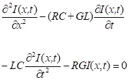
The system under analysis is a relationship between the atmosphere and the earth, represented as a cylindrical condenser. The separation between these entities is defined by a discharge channel, which is assumed straight and without deviations. The cylindrical condenser has a distance of 1 km between its components, while the discharge channel has a diameter of approximately 20 cm. During the simulation of this scenario, a characteristic altitude of 1000 m is considered. This altitude is divided into 250 segments, each with a time interval Δt of 0.5 µs, for a detailed representation of the process. The system of equations used in this work is the one proposed in references ¹and ² from which (1) and (2) are extracted as main equations

where Vx,tis the cloud voltage, Ix,t is the discharge current and R, L, C y G are the resistance of the channel, the inductance associated with the discharge, and the inductance associated with the discharge, Cthe capacitance and G the conductance, respectively. Combining equations (1) and (2) yields the well-known telegrapher's equation for current:

(3)

is easy to show that equation (3) has the same form for the lightning voltage. In this case, it is solved numerically to determine the return discharge current with the appropriate initial and boundary conditions. In addition to the actual parameters that allow the atmospheric discharge to be accurately described, it should be noted that this equation has been solved on other occasions, and the authors make assumptions that greatly simplify it ⁶.

III. NUMERICAL DEVELOPMENT AND IMPLEMENTATION

For the discretization of equation (3), the basic idea of finite differences is to replace continuous space-time with a discrete set of points. The time step between two consecutive levels is denoted ∆t, and the distance between two adjacent points in space ∆x ³.

The next step is to replace the differential equations with discrete equations. This is achieved by approximating the differential operators by their corresponding finite differences and considering the function values at adjacent points in the mesh. In this way, an algebraic equation is obtained at each point of the grid for each term of the differential equation. These equations involve the function values at the moment considered and their nearest neighbors. Using the approximations obtained by Taylor's series development, its corresponding discretization replaces each differential operator in equation (3), and the following is obtained.

This equation has the property that it involves only two values of the wave function at the last time level; the value , then, can be cleared in terms of values at previous times to obtain the equation of the discretized telegrapher, which will later be implemented in Matlab.

To numerically implement this equation, it is necessary to specify the boundary and initial condition. The current in the cloud is assumed to be a constant value taken as zero. Therefore, the cofounder's condition is

(5)

Where h is the height of the cloud where the discharge starts, at t = 0, the current distribution is assumed to be a constant value. Therefore, the initial condition is

(6)

A. The Algorithm

The algorithm for finding the numerical solution is described in Figure 1.

Source: Authors.

Figure 1 The algorithm for finding the numerical solution. 

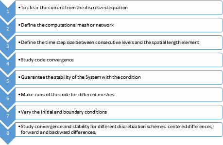
Equation (4) is implemented numerically in MATLAB. In the case of the telegrapher's equation, the input parameters R, L, C, and G are needed, which are assumed to be known in the discharge channel. The values used in this case are shown in Table 1.

Tabla 1 Electrical parameters of the discharge channel of an ATDI. These parameters were varied to validate the code, and the impact on the solutions was not representative. 

Heigh (x)	1000 m
Inductance (L)	2.18 Mh
Capacitance (C)	6.95 Pf
Conductance (G)	5 Us
Resistance (R)	1000 to 5000 ohms

B. Stability and convergence analysis

For any simulation, stability and convergence tests are necessary, among other aspects, because of the following ^3,4,5:

• When applying finite difference methods involving numerical solutions of second-order differential equations, in addition to considering errors due to rounding and series truncation, it is essential to remember that finite difference expressions are derived from a Taylor series approximation up to the second term. This approximation introduces an error in the calculations that need to be controlled.

• There are also errors associated with the limitations of fitting the physical model to accurately describe the natural system and the constraints imposed by the boundary conditions. Convergence and stability validation verify the correctness of the approximations made by finite differences in the discretization process.

• Methods are available to evaluate the convergence of a code when analytical solutions are known. In this study, the electrical parameters are considered to achieve a sufficiently refined mesh, thus allowing code convergence in as few iterations as possible. To achieve this, the CFL condition is applied to ensure that the mesh will enable us to obtain a solution closer to reality.

• A particular case arises when time-stepping schemes are used as a numerical solution method. Consequently, in many simulations, the time step must be smaller than a characteristic value to prevent the code from becoming unstable and producing incorrect results. This constraint is commonly called the numerical propagation speed in the CFL condition.

• To assess stability, it is sufficient to ensure that the solutions of the differential equations do not exhibit oscillations, which can be determined by observing the graphs representing the time evolutions. This requires allowing the time-dependent variables to evolve over a prolonged period to verify that they do not exhibit unexpected oscillations or fluctuations.

• Convergence refers to how the numerical solution approaches a known or actual analytical solution. In situations where the analytical solution is unknown, it is possible to use an iterative approach to evaluate convergence. The numerical value of the first iteration is used as the analytical approximation and compared to the numerical value of the second iteration. Then, the value of the second iteration is taken as the analytical approximation and compared with the numerical value of the third iteration, and so on. This approach constitutes one of the tests implemented to validate the code in this study.

To converge the code, we proceeded as follows: since the finite difference approximation method used in the Taylor series development is of second order, we postulate that the error is also of second order at ∆x:

Error=∆x2                            (7)

By applying logarithm and its properties to both members of the equation (7):

log⁡Error=2log⁡∆x                  (8)

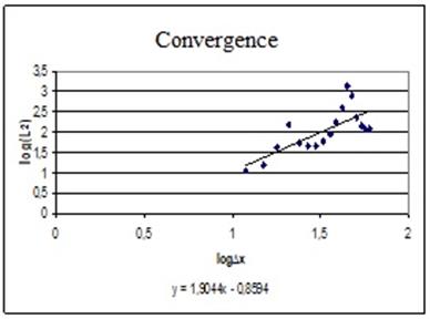
Equation (8) has a line of slope equal to two. If from the graph log⁡Error Vs log⁡(∆x)the error between a known analytical solution and the numerical solution found for equation (4) is obtained. A slope approximately equal to two implies that the numerical solution converges to the analytical solution. In this case, a general expression for the convergence calculation given by the L₂ norm was used for convergence ^3,4,11

L2=∑i,jfij-Fij2                  (9)

Where f_ij is the analytical solution, and F_ij is the numerical solution obtained, and L₂ = Error. Figure 2 shows the two current wave models used to perform this convergence. That is the analytical solution and the numerical solution obtained.

Figure 2 Numerical and analytical discharge current waveforms. 

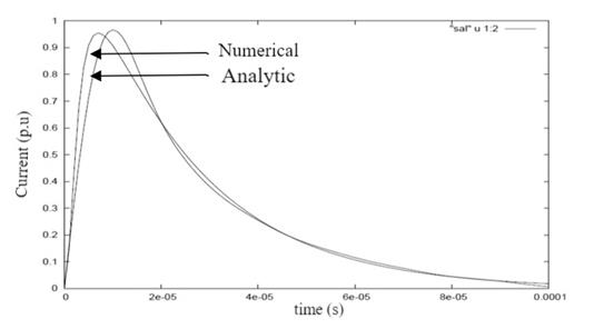
The waveform generated with the Heidler function ^8,9,10was selected as the analytical solution and compared with the numerical solution of the telegrapher's equation to estimate the convergence error. Figure 3 shows a line of average slope m=1.9 using least squares for linear regression, with differential steps of 3 microseconds. The numerical solution converges to the analytical solution to the second order of approximation.

Figure 3 Result of the average line using least squares for convergence. 

The particular case of a lossless line (R=G=0) leads to a differential equation identical to the string equation and whose algorithm is straightforward to implement numerically.

∂2V(x,t)∂x2=LC∂2V(x,t)∂t2               (10)

∂2Ix,t∂x2=LC∂2Ix,t∂t2                (11)

So that you know, the solution of equations (10) and (11) can be used to verify the convergence of the code in the limits of R=G=0. To verify the validity of the solution of the telegrapher's equation (3), in codes where the equation is solved with R=G=0, the current's numerical solution coincides with that of equation (11). A mesh refinement was performed for N=1000, 10000, 200000, and 1000000, and the code remained stable and convergent for all meshes, only with the centered finite difference scheme. With the forward and backward finite difference schemes, the code is unstable for coarse, medium, and fine meshes.

IV. RESULTS

Another test and validation of the code elaborated in MATLAB was a series of tests performed on the code by varying the parameters. A series of plots are shown for G=0 and G≠0 for different numbers of points to change the size of the spatial differentials and test the previously exposed stability criteria. The fact that the conductance parameter is zero implies non-real solutions since there are losses in the real lines. Meanwhile, when G≠0, the solutions are closer to reality. In the case of Figure 4, for several points N≥1000, the code starts to break the CFL condition, and oscillations are appreciated, representing an atypical behavior for a phenomenon of these characteristics. For a N≤200, the CFL condition (ratio between Δt and Δx) is violated.

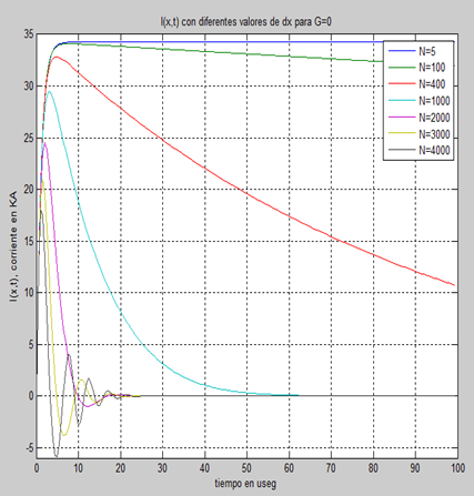
Figure 4 Numerical solution for different values of the number of mesh points N and the conductance parameter, G=0. 

Figure 5 compares the waves obtained numerically with the code in Matlab (both for G=0 and G≠0) and the analytical solution. It can be noticed the difference with G=0. This is because the discharge channel's dissipative characteristics are not considered. The solutions closest to reality are obtained when G≠0.

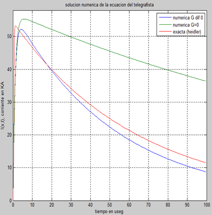
Figure 5 Comparison between the numerical solutions for the conductance parameter G=0 and G≠0 and the analytical solution (Heidler). This plot was obtained with a run of the program in Matlab. 

Once the implemented numerical solution was compared with the analytical solution and the codes were validated, we simulated different models. Figure 6 shows the current calculated from Equation (3) for different values of G. In all cases, the start-up time and the differentials were the same. What differentiates them is the attenuation and the stability of the code.

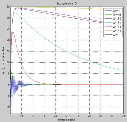
Figure 6 Numerical solution for the discharge current with different values of the conductance parameter G. 

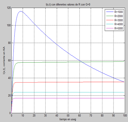
Figure 7 shows a series of plots for different values of the discharge channel resistance, R, both for G=0, to simulate the different resistivities present in the atmosphere by having areas with higher humidity and pollution than others.

Figure 7 Numerical solution with different values of channel resistance R and conductance parameter G=0. 

CONCLUSIONS